install.packages("tidyverse")R advanced: packaging and sharing functions
The strength of the R programming language lies in the endless possibilities custom functions can bring, and a community of users who happily share their contributions with peers.
This session is directed at intermediate to advanced R users wanting to learn about creating, packaging and sharing functions.
In this session, you will learn about:
- creating new custom functions
- packaging your functions into a cohesive collection
- properly documenting your code
- versioning your code
- using online services to share your package
- using RStudio features that make life easier
Setting up
Download the project
So we can get straight into the interesting stuff, we have an R project that already contains relevant custom functions: download the archive.
Unzip this archive, and open the .Rproj file to open the project in RStudio.
Install packages
Let’s make sure we have the whole Tidyverse packages ready. If you don’t have them installed on your computer just yet, run this command in the Console:
Create a script
Create a new script by using the New File menu (first icon in the toolbar) and selecting “R Script”.
How to build a function
In R, once we find we are limited by the functions available (in both R and in packages available online), there always is the possibility of designing our own functions.
This is what a basic function definition looks like:
human_age <- function(dog_age) {
  dog_age * 7
}
Here, we create a custom function that will take the age of a dog, and convert it to human years.
We need to:
- give the function a name (just like when we create an object)
- specify which arguments are available when the function is used
- define what happens when the function is called, in between the curly braces
{}
After executing this block of code, we have defined our function, and we can see it listed in the Environment panel. We can now use it just like any other function:
human_age(12)[1] 84As you can see, functions will by default return the last evaluated element.
Our example ACORN data
Let’s have a look at our pre-defined functions now.
The data that we want to deal with comes from the Bureau of Meteorology website. You can find more information about it here: http://www.bom.gov.au/climate/data/acorn-sat/#tabs=Data-and-networks
This project provides temperature data for 112 Australian weather stations. We want to use the maximum daily temperature data, which means we will have to deal with 112 separate CSV files.
Download the data
We will use a custom function that downloads the data. Because the data is provided as a zipped archive, we need to do two things in the body of our function:
- download the archive from the relevant URL (with
download.file()) - unzip it into a directory (with
untar())
Open the “get_acorn.R” file from the Files panel, and look at the code it contains:
get_acorn <- function(dest) {
  # download the archive of station data from BOM
  download.file(url = "ftp://ftp.bom.gov.au/anon/home/ncc/www/change/ACORN_SAT_daily/acorn_sat_v2.5.0_daily_tmax.tar.gz",
                destfile = "acorn_sat_v2.5.0_daily_tmax.tar.gz")
  # extract it into a directory
  if (!dir.exists(dest)) {
    dir.create(dest)
  }
  untar(tarfile = "acorn_sat_v2.5.0_daily_tmax.tar.gz",
        exdir = dest)
}
The only argument we make available in the function is the dest argument: the destination of the files, i.e. the name of the directory where we want to store the files.
See the if statement? We are using branching: if the directory does not exist, it will be created. If it already exist, it will move on to the next step without executing the dir.create(dest) command.
To have access to this new funtion, make sure you execute the whole block of code. Back in our script, we can now call our new function to get the data:
get_acorn(dest = "acorn_data")We now have the 112 CSV files. How do we import and clean one single station’s data?
Read a single file
The package readr provides a read_csv() function to import data from a CSV files.
We will use several tidyverse packages, so we might as well load the core Tidyverse packages.
library(tidyverse)
read_csv("acorn_data/tmax.001019.daily.csv")
Looks like we need to fill down the station ID, then remove the first row, which we can do by piping extra fill() and slice() steps:
read_csv("acorn_data/tmax.001019.daily.csv") |>
  fill(3) |> # fill down station ID
  slice(-1) # remove the first row
We also want to remove the superfluous column, and rename the maximum temperature variable, which can be done in one go with the select() function:
read_csv("acorn_data/tmax.001019.daily.csv") |>
    fill(3) |> # fill down station ID
    slice(-1) |>  # remove first row
    select(date, station = 3, max.temp = 2) # keep interesting columns
This is probably the data we want to end up with when reading a file.
Have a look at the function defined in “read_station.R”:
read_station <- function(file) {
  read_csv(file, # read the CSV
           show_col_types = FALSE) |> # be more quiet
    fill(3) |> # fill down station ID
    slice(-1) |>  # remove first row
    select(date, station = 3, max.temp = 2) # keep interesting columns
}
This is pretty much the steps we used before, made into a function. The only argument is file, to provide the name of the file we want to read.
Note also the extra argument show_col_types = FALSE used to suppress noisy messages.
Make sure you define this function by executing the code. You can also use the “Source” button at the top right of the source panel.
Back in our script, we can now test it on our first file:
read_station("acorn_data/tmax.001019.daily.csv")It is often useful to define functions in a separate script to the data analysis script. Know that you can then “source” those custom functions at the beginning of the analysis script thanks to the
source()function.
Read and merge all the data
We now want to iterate over all the files, and create a single merged dataframe.
We can start with finding all the relevant files in the data directory:
files <- list.files(path = "acorn_data", # where to look
           pattern = "tmax*",                         # what to look for
           full.names = TRUE)                         # store full path
See that files is a character vector containing the name of 112 files?
We can then apply our custom function iteratively to each file. For that, purrr’s map_ function family is very useful. Because we want to end up with a dataframe, we will use map_dfr():
We now have close to 4 million rows in our final dataframe all_tmax.
We might also want to create a function from the two previous steps, so we only have to provide the name of the directory where the CSV files are located. That’s what we have in the “merge_acorn.R” file:
merge_acorn <- function(dir) {
  files <- list.files(path = dir,
           pattern = "tmax*",
           full.names = TRUE)
  map_dfr(files, read_station)
}
Let’s source this function, and try it in our script:
all_tmax <- merge_acorn("acorn_data")This does the same as before: we have a final merged dataset of all the max temperatures from ACORN.
Making functions more resilient
We can make our functions more resilient by adding stop() and warning() calls.
For example, what if our merge_acorn() function is not provided with a valid path?
merge_acorn("blah")We could improve our function with an if statement and a stop() function:
merge_acorn <- function(dir) {
  if (!dir.exists(dir)) {
    stop("the directory does not exist. Please provide a valid path as a string.")
  }
  files <- list.files(path = dir,
           pattern = "tmax*",
           full.names = TRUE)
  map_dfr(files, read_station)
}
Now, let’s see what happens if we don’t provide a valid directory:
merge_acorn("bleh")This will neatly stop our function and provide an error message if the path is not found.
Use the data
Let’s have a look at a summary of our data:
summary(all_tmax)Now that we have very usable data, why not create a visualisation? For example, let’s have a look at how the yearly mean of max temperatures evolved over the years:
mean_max <- all_tmax |>
  filter(!is.na(max.temp)) |>              # remove rows with missing temperature
  group_by(year = year(date), station) |>
  filter(n() > 250) |>                     # keep station-years with enough data
  summarise(max.temp = mean(max.temp)) |>  # by year and station
  summarise(max.temp = mean(max.temp), n_stations = n()) # by year only

ggplot(mean_max, aes(x = year, y = max.temp)) +
  geom_point(aes(colour = n_stations)) +   # colour the points by number of sites
  geom_smooth() +                          # trend line
  labs(y = "Yearly max temp average (°C)") +
  theme_minimal()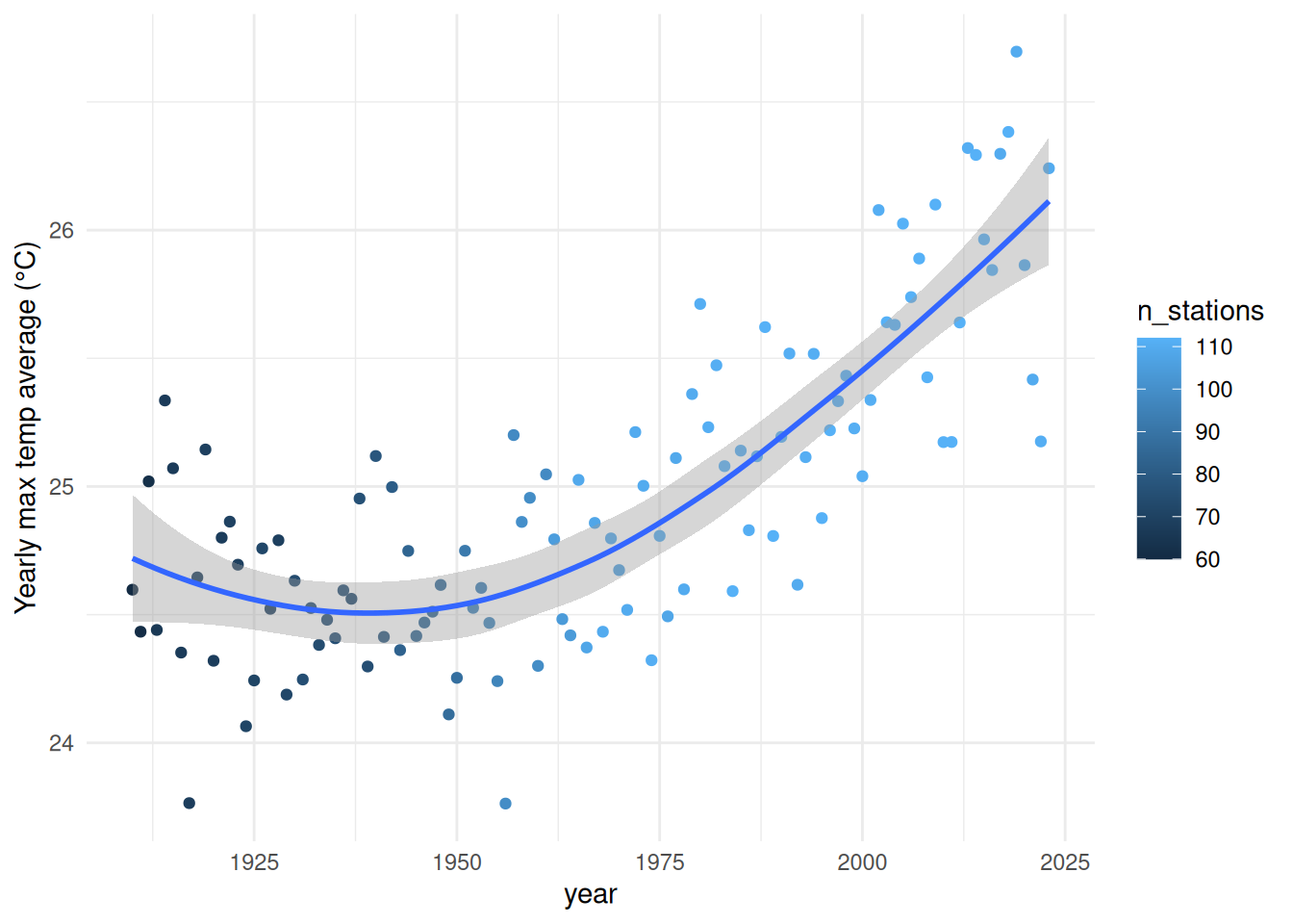
We now want to share our useful functions with the World!
Packaging functions
Some useful packages for package development: devtools, usethis, roxygen2
To prepare for packaging our functions, we would ideally have them in separate scripts named after the function they define, which is already the case for our three functions: “get_acorn.R”, “read_station.R” and “merge_acorn.R”.
Now, let’s create a new project for our package, to keep things tidy: File > New Project… > New Directory > R Package.
Let’s name our package “acornucopia”.
We can pick the three function scripts we created before as the base for our package.
We end up with a basic package structure:
- DESCRIPTION
- man
- NAMESPACE
- R
Let’s go through those main components.
1. Description
This is the general description of the what the package does, who developed and maintains it, what it needs to work, and what licence it is released under.
The file already contains a template for us to fill in. We can update the fields with relevant information, in particular for Title, Author, Maintainer, Description and License:
Package: acornucopia
Type: Package
Title: Process ACORN data
Version: 0.1.0
Author: Your Name
Maintainer: Your Name <yourself@somewhere.net>
Imports: readr, dplyr, purrr
Description: Functions to import, cleanup and merge temperature data from ACORN stations
License: GPL-3
Encoding: UTF-8
LazyData: true
Notice that we added the Imports: field. This allows us to specify what extra packages are needed for our package to work.
Which licence?
GPL or MIT are common licences for R packages. They are Open Source and allow others to reuse your code, which is the norm in the R ecosystem. However, they differ in how much can be done when creating a derivative: MIT is more “permissive” in that it allows creating closed source derivatives, whereas GPL is more “viral” in that only compatible open source licences can be used. To help you pick one, try the “Choose a License” website.
2. NAMESPACE
The NAMESPACE file lists the functions available to the user when the package is loaded with library().
By default, it uses a regular expression that will match anything with a name that starts with one or more letters (in the R directory).
3. R
This is where our function definitions go. If you haven’t imported the three scripts when creating the package project, copy and paste them in now.
Documenting functions
We are using the package roxygen2 to document each function.
With a function’s R script open in the source pane, and your cursor inside the function’s code, go to Code > Insert Roxygen Skeleton. This will add a template above your function, which can be used to generate the function’s documentation. You can see that it is adapted to your code. For example, for the read_station() function:
#' Read a station's CSV file
#'
#' This function imports and cleans a single ACORN station CSV file.
#'
#' @param file Path and filename of CSV file to read (as a string)
#'
#' @return A clean tibble
#' @export
#' @import dplyr
#' @importFrom readr read_csv
#' @examples
#' \dontrun{
#' read_station("path/to/file.csv")
#' }- up the top, the first sentence is the title, and the following paragraph gives a description. A third section can be used to give more details.
@exportcan be used as is to populate the NAMESPACE file with this function- we added the
@importand@importFromtags to specify precisely what package or functions need to be imported for our function to work. \dontrun{}can be used for examples that will not work, or that shouldn’t be executed for a variety of reasons.
Pressing Return inside the Roxygen skeleton will automatically prepend the necessary comment characters
#'
We can then generate and view the help file with:
devtools::document()
?read_station
Notice that we get a warning about NAMESPACE not being generated by roxygen2. If we want roxygen2 to take care of this file, we can first delete it, and then run the document() function again.
NAMESPACE is now populated with the exports and imports defined in the Roxygen documentation.
Challenge 1: document a function
Use roxygen2 to create the documentation for merge_acorn(). Try generating the documentation again, and check your NAMESPACE.
Testing the package
At any time, we can load the package to test its functions:
Ctrl + Shift + L
And to check our package for issues, we can use the “Check” button in the Build tab, or the following command:
devtools::check()This function does a very thorough check, and will take some time to go through all the steps.
Notice any error, warning or note?
Building and installing
We can also install our package on our system.
The easiest way is with the “Install and Restart” button. This will list the package in your Packages tab, which means you will be able to load it whenever you need the functions when you work on another project.
However, if you want to save a copy and share it with others, you can build the package:
- On Windows: Build > Build Binary Package
- On Linux or macOS: Build > Build Source Package
The resulting archive is what you can share with colleagues and friends who want to try your package on their computer.
To install it (the name of the archive will depend on your system), either use the “Install” menu in the Packages tab (using “Install from Package Archive File” instead of the CRAN repositories), or use this command:
install.packages("../acornucopia_0.1.0.tar.gz", repos = NULL)We have to set
repostoNULLso R doesn’t look for the package on CRAN.
Others can now have our package listed in their packages list, ready to be loaded whenever they want to use its functions.
Best practice
As a general rule, it is best to stick to a minimum of dependencies, so the package:
- requires less maintenance
- is lighter to install
For function names, try to avoid dots, and use underscores instead (tidystyle).
Publishing
We can then try to publish our package, making sure that we follow the guidelines / requirements relevant to where we publish it.
In order to publish on CRAN, we have to follow stringent policies: https://cran.r-project.org/web/packages/policies.html
Although CRAN is the main and default repository for the R ecosystem, other repositories and communities exist. For example, Bioconductor hosts thousands of packages relevant to bioinformatics, and ROpenSci supports a community around hundreds of peer-reviewed packages useful for querying and analysing various scientific data sources.
Using version control
When developing software, it is important to keep track of versions, and if you collaborate with others, of authors too.
It also allows you to roll back to a previous version if needed.
RStudio integrates Git, the most popular version control system for software development. To setup a Git repository for our package, we can use “Tools > Version Control > Project Setup…”, and create a new Git repository. We can then use the Git tab to save snapshots of our files.
You can then host your code on Gitlab or GitHub to make it accessible to others. See for example: https://github.com/Lchiffon/wordcloud2
The package usethis provides many useful functions to setup packages, including a use_github() function to quickly create a remote repository, and a use_readme_*() to add a readme file for the project.
Others will then be able to install your package from your remote repository with:
devtools::install_github("username/myPackage")
devtools::install_gitlab("username/myPackage")
Useful links
- R Packages, by Jenny Bryan and Hadley Wickham: http://r-pkgs.had.co.nz/
- Full official guide for packaging: https://cran.r-project.org/doc/manuals/r-release/R-exts.html
- What to lookout for when publishing to CRAN: https://cran.r-project.org/web/packages/policies.html
- Package development cheatsheet: https://github.com/rstudio/cheatsheets/raw/master/package-development.pdf
Extras
These two topics are important when developing custom functions, but can not fit in this session. They are described here for reference, if needed.
Quasiquotation
Tidyverse packages use quasiquotation and lazy evaluation to save us a lot of typing.
For example, we can do:
mtcars |> select(disp)… but disp is not an existing object in our environment.
quo_name() quotes, whereas sym() gets the symbol.
Try eval(sym(something)).
This might lead to issues, like:
selector <- function(d, col) {
  d |> select(col)
}
We need to quote-unquote:
selector <- function(d, col) {
  col <- enquo(col) # do not evaluate yet!
  d |> select(!!col) # evaluate here only
}
For multiple arguments:
selector <- function(d, ...) {
  col <- enquos(...)
  d |> select(!!!col)
}
Classes
We can assign new classes to objects:
obj <- "Hello world!"
class(obj) <- "coolSentence"
attributes(obj)
The structure() function is useful for that too.
We can then define methods for this specific class, for example a coolSentence.print() function.