Python training (1 of 4): The Fundamentals

Recent update: Positron

These materials have recently been updated to reflect our shift from Spyder to the Positron IDE.

Positron looks and feels like VS Code with the data science features of RStudio and Spyder.

The Python content remains unchanged.

This hands-on programming course – directed at beginners – will get you started on using Python 3 and the program Positron to import, explore, analyse and visualise data.

Setup

You’ll need to install Python 3 and Positron (or your preferred IDE). This depends on your machine (and your admin rights).

If you can, download and install Python with the official install manager. If you don’t have admin rights, you should still be able to perform a user-based install.

Next, download and install Positron.

You should install Positron via Company Portal / Self-service. If Positron cannot detect a Python interpreter, you should install Anaconda as well.

You should install Positron via Zenworks. If Positron cannot detect a Python interpreter, you should install Python with IDLE as well.

Introducing Python and Positron

Python is a programming language that can be used to build programs (i.e. a “general programming language”), but it can also be used to analyse data by importing a number of useful modules.

We are using Positron to interact with Python more comfortably. If you have used RStudio to interact with R before, you should feel right at home: Positron is a program designed for doing data science with Python and built by the RStudio developers (Posit).

We will start by using the console to work interactively. If Positron hasn’t started with Python (it might have automatically loaded R!), you should “Start new session” or click on the R version button (top right of console) and change it to Python.

This is our direct line to the computer, and is the simplest way to run code. You know it’s the console by the distinctive prompt:

>>>

which awaits your command.

Maths

To start with, we can use Python like a calculator. Type the following commands in the console, and press Enter to execute them:

After running each command, you should see the result as an output.

Variables

Numbers

Most programming languages are like spoken language in that they have nouns and verbs - you have “things” and they “do things”. In Python, we have variables and functions. We’ll look first at variables, the nouns of Python, which store data.

To create a variable, we choose its name (e.g. favNumber) and assign (=) it a value (e.g. 42):

example_int = 42

You can then retrieve the value by running the variable name on its own:

example_int

Notice that, in the variable explorer, the number has also appeared? This is one way that Positron helps you program.

Let’s create more variables. We can use the variable names in place of their values, so we can perform maths:

example_float = 5.678
example_int * example_float

238.476

In the variable explorer, the type of example_int is int (far right), while the other is float. These are different variable types and can operate differently. int means integer, and corresponds to whole numbers, while float stands for floating point number, meaning decimals. You may occasionally encounter errors where you can only use one type.

Booleans

Even simpler than integers is the boolean type. These are either 1 or 0 (True or False), representing a single binary unit (bit). Don’t be fooled by the words, these work like numbers: True + True gives 2.

example_bool = True

In Python, the boolean values True and False must begin with a capital letter.

Sequences

Let’s look at variable types which aren’t (necessarily) numbers. Sequences are variables which store more than one data point. For example, strings store a sequence of characters and are created with quotation marks '<insert string>' or "<insert string>":

example_string = 'Hello world!'

We can also create lists, which will store several variables (not necessarily of the same type). We need to use square brackets for that:

example_list = [38, 3, 54, 17, 7]
diverse_list = [3, 'Hi!', 9.0]

Lists are very flexible as they can contain any number of items, and any type of data. You can even nest lists inside a list, which makes for a very flexible data type.

Operations on sequences are a bit different to numbers. We can still use + and *, but they will concatenate (append) and duplicate, rather than perform arithmetic.

example_string + ' How are you?'
example_list + diverse_list
3 * example_list

[38, 3, 54, 17, 7, 38, 3, 54, 17, 7, 38, 3, 54, 17, 7]

However, depending on the variable, some operations won’t work:

example_string + example_int

---------------------------------------------------------------------------
TypeError                                 Traceback (most recent call last)
Cell In[9], line 1
----> 1 example_string + example_int

TypeError: can only concatenate str (not "int") to str

There are other data types like tuples, dictionaries and sets, but we won’t look at those in this session. Here’s a summary of the ones we’ve covered:

Category	Type	Short name	Example	Generator
Numeric	Integer	`int`	`3`	`int()`
Numeric	Floating Point Number	`float`	`4.2`	`float()`
Numeric	Boolean	`bool`	`True`	`bool()`
Sequence	String	`str`	`'A sentence '`	`" "` or `' '` or `str()`
Sequence	List	`list`	`['apple', 'banana', 'cherry']`	`[ ]` or `list()`

The generator commands are new. We use these to manually change the variable type. For example,

int(True)

yields 1, converting a boolean into an integer. These commands are functions, as opposed to variables - we’ll look at functions a bit later.

Indexing

We can access part of a sequence by indexing. Sequences are ordered, starting at 0, so the first element has index 0, the second index 1, the third 2 and so on. For example, see what these commands return:

example_string[0]
example_string[6]
example_list[4]

If you want more than one element in a sequence, you can slice. Simple slices specify a range to slice, from the first index to the last, but not including the last. For example:

example_list[0:4]

[38, 3, 54, 17]

That command returns elements from position 0 up to - but not including! - position 4.

Scripts and folders

So far, we’ve been working in the console, our direct line to the computer. However, it is often more convenient to use a script. These are simple text files which store code and run when we choose. They are useful to

write code more comfortably,
store clearly defined steps in chronological order,
share a process with peers easily, and
make your work reproducible

Let’s create a folder system to store our work and navigate there.

Create a new folder on your computer called “python_training” (or something similar).
Press File > Open folder..., find and select the new folder

Positron will now move to the new folder.

Create a new script with New > New file... and choose “Python file”
Save the file to give it a name (e.g. fundamentals.py)

You should now see a script on the explorer pane in Positron, looking something like this:

Try typing a line of code in your new script, such as

1 + 1

Press ctrl+enter to run each line (or CMD+return). You should see the same code appear in the console with its result.

Functions

Functions are little programs that do specific jobs. These are the verbs of Python, because they do things to and with our variables. Here are a few examples of built-in functions:

example_list = [1,2,3,4]
len(example_list)
min(example_list)
max(example_list)
sum(example_list)
round(5.123)

Functions always have parentheses after their name, and they can take one or several arguments, or none at all, depending on what they can do, and how the user wants to use them.

Here, we use two arguments to modify the default behaviour of the round() function:

round(5.123, 2)

5.12

Notice how Positron gives you hints about the available arguments after typing the function name?

Operators

Operators are a special type of function in Python with which you’re already familiar. The most important is =, which assigns values to variables. Here is a summary of some important operators, although there are many others:

General

Operator	Function	Description	Example command
=	Assignment	Assigns values to variables	`a = 7`
#	Comment	Excludes any following text from being run	`# This text will be ignored by Python`

Mathematical

Operator	Function	Description	Example command	Example output
+	Addition	Adds or concatenates values, depending on variable types	`7 + 3` or `"a" + "b"`	`10` or `'ab'`
-	Subtraction	Subtracts numerical values	`8 - 3`	`5`
*	Multiplication	Multiplies values, depending on variable types	`7 * 2` or `"a" * 3`	`14` or `'aaa'`
/	Division	Divides numerical vlues	`3 / 4`	`0.75`
**	Exponentiation	Raises a numerical value to a power	`7 ** 2`	`49`
%	Remainder	Takes the remainder of numerical values	`13 % 7`	`6`

Comparison

Operator	Function	Description	Example command	Example output
==	Equal to	Checks whether two variables are the same and outputs a boolean	`1 == 1`	`True`
!=	Not equal to	Checks whether two variables are different	`'1' != 1`	`True`
>	Greater than	Checks whether one variable is greater than the other	`1 > 1`	`False`
>=	Greater than or equal to	Checks whether greater than (>) or equal to (==) are true	`1 >= 1`	`True`
<	Less than	Checks whether one variable is less than the other	`0 < 1`	`True`
<=	Less than or equal to	Checks whether less than (<) or equal to (==) are true	`0 <= 1`	`True`

Finding help

To find help about a function, you can use the help() function, or a ? after a function name:

help(max)
print?

Help on built-in function max in module builtins:

max(...)
    max(iterable, *[, default=obj, key=func]) -> value
    max(arg1, arg2, *args, *[, key=func]) -> value
    
    With a single iterable argument, return its biggest item. The
    default keyword-only argument specifies an object to return if
    the provided iterable is empty.
    With two or more arguments, return the largest argument.

The help information can often be dense and difficult to read at first, taking some practice. In the next session we look closer at interpreting this documentation, one of the most important Python skills.

For a comprehensive manual, go to the official online documentation. For questions and answers, typing the right question in a search engine will usually lead you to something helpful. If you can’t find an answer, StackOverflow is a great Q&A community.

Activity 1

In this first activity, write a program which takes an age in years and outputs how many minutes they’ve lived for. Note that

\[\text{Age (minutes)} = \text{Age (years)} \times 365 \times 24 \times 60\]

Steps

Store the age in years in a variable
Calculate the age in minutes
Print a message with the output

Note: if you want to print a number (e.g. the age), the easiest way is to send multiple arguments to the print function. For example, print("The first number is", 1)

Advanced

If this is too easy, try to get the user to provide their age themselves with the command int(input(...)). Make sure to use int(), otherwise the string multiplication will may cause a crash. You’ll want the documentation for input().

Solution

We have three lines of code corresponding to the steps above:

### Age in minutes calculator
  
# Input age
age_years = 56

# Calculate age in mins
age_mins = age_years * 365 * 24 * 60

# Print result
print("You have lived for", age_mins, "minutes!")

You have lived for 29433600 minutes!

To include the input() command,

### Age in minutes calculator
  
# Input age
age_years = int(input("What is your age? "))

# Calculate age in mins
age_mins = age_years * 365 * 24 * 60

# Print result
print("You have lived for", age_mins, "minutes!")

Packages

Python is set apart from other languages by the scale of its community packages and the ease with which you import them. While you could code everything you need from scratch, it’s often more effective to import someone else’s predefined functions.

Built-in packages

Python comes with a number of pre-installed packages, so they’re already on your computer. However, your specific Python application doesn’t have access to them until they’re imported:

import math

The module math brings in some mathematics constants and functions. For example, you will get an error if you run pi on its own, but we can access the constant using the module:

math.pi
2*math.pi
math.cos(math.pi)

-1.0

Note that we use a period . in order to access objects inside the module. In general, we use periods in Python to access objects stored inside other objects.

Naming

Some modules have long names and use abbreviated nicknames when imported.

import math as m
m.pi

3.141592653589793

Here the module math is stored as m in Python.

Where this naming is used, it is usually the standard, and sharing code with different (including original/full) module names will not be compatible with other programmers.

Common external packages

There are hundreds of thousands of external packages available. These do not normally come with Python installations (although they do often come with Anaconda-based installations).

While the import command lets you connect your Python script with a module on your computer, you’ll need to download and install the package first.

The simplest way to do this is with the pip bash command. This is not a Python command: it is a separate program that you run in a terminal. Positron gives us a bit of beyond-Python magic to run it in the console anyway:

%pip install <package_name>

We recommend that you run this in the console directly, not in your script. Just because you only run it once per Python installation.

If you are running this directly the terminal (not the console), you should drop the %:

pip install <package_name>

Beware Anaconda (conda) users

If you’ve installed Python via the Anaconda distribution, you should avoid using pip to install packages where possible. This is because you can create conflicts with conda-based packages. However, all the packages for today should already be installed, so you can skip this step!

Anaconda provides an alternative interface to pip for installing packages:

conda install <package_name>

which you should preference. Only use pip if the package is not accesible via conda.

We’ll look at a few packages today, and a few more as we progress through the series. The ones for today are

numpy (for numerical operations, linear algebra etc.)
pandas (for panel data, e.g. csv files, spreadsheets etc.)
seaborn (for high-level visualisations)

To install them all in one go, use

%pip install numpy pandas seaborn

Once you’ve installed the packages, you will need to restart the console with the Restart Python button in the console.

An example: `numpy`

You might recall that multiplication for sequences replicates them. This makes multiplying numeric lists unexpected:

3 * [1,2,3]

[1, 2, 3, 1, 2, 3, 1, 2, 3]

What if we wanted to multiply each element by 3? Well, the developers of numpy decided to create a variable where this does happen: the array. To turn a list into an array, use the np.array() function

import numpy as np
example_array = np.array([1,2,3])

3 * example_array

array([3, 6, 9])

That works well!

Some popular packages include

Package	Install command	Import command	Description
NumPy	`pip/conda install numpy`	`import numpy as np`	A numerical Python package, providing mathematical functions and constants, vector analysis, linear algebra etc.
Pandas	`pip/conda install pandas`	`import pandas as pd`	Panel Data - data transformation, manipulation and analysis
Matplotlib	`pip/conda install matplotlib`	`import matplotlib.pyplot as plt`	Mathematical ploting library, a popular visualisation tool. Note that there are other ways to import it, but the `.pyplot` submodule as `plt` is most common.
Seaborn	`pip/conda install seaborn`	`import seaborn as sns`	Another visualisation tool, closer to ggplot2 in R, built upon a matplotlib framework.
SciPy	`pip/conda install scipy`	`import scipy` or `import scipy as sp`	A scientific Python package with algorithms and models for analysis and statistics.
Statsmodels	`pip/conda install statsmodels`	`import statsmodels.api as sm` and/or `import statsmodels.tsa.api as tsa`	Statistical modelling. The first import `sm` is for cross-sectional models, while `tsa` is for time-series models.
Requests	`pip/conda install requests`	`import requests`	Make HTTP (internet) requests.
Beautiful Soup	`pip/conda install beautifulsoup4`	`from bs4 import BeautifulSoup`	Collect HTML data from websites.

Activity 2

In this final activity, we’re going to create some sample data and visualise it.

Our goal is to import and visualise random BMI data

We’ll complete this in two parts. Before we begin, we need to set things up by importing the modules we need

import pandas as pd
import seaborn as sns

If importing any of these causes an error, it could be because you haven’t installed it yet. See above for information on how to do so.

Before we begin this activity we should bring in the data. To do this, we use the pd.read_csv() function, specifying the file path as the first argument (this can be a URL), and store it in a variable (typically df). For example,

df = pd.read_csv("insert_filepath_here")

Today’s data is five (random) people’s height and weight. You can download it here.

Create a folder called data next to your script
Download the data
Move the csv into your data folder
Read it in with df = pd.read_csv("data/BMI_data.csv")

Part 1: Modifying the data

For the first part of the challenge, you’ll need to compute each person’s BMI, and store it in a new column. For reference, we access columns by indexing based on their name, e.g. df["Weight"] is the Weight column. To make a new column, we pretend that it already exists and assign into it. For example, to convert from kilograms to pounds,

# Create a new column called Weight (lb) and store the weight in pounds
df["Weight (lb)"] = df["Weight"]*2.205

To compute the BMIs, make another new column and use the following formula to calculate the BMI.

\[ \text{BMI} = \frac{\text{Weight (kg)}}{(\text{Height (m)})^2} \]

It should look something like

df["BMI"] = ...

Hint: \(x^2\) is x**2

Once you’ve done these steps, you should see the following:

	Names	Height	Weight	Weight (lb)	BMI
0	Alice	1.90	94	207.27	26.038781
1	Bob	1.81	102	224.91	31.134581
2	Charlie	1.87	108	238.14	30.884498
3	Dilsah	1.88	84	185.22	23.766410
4	Eliza	1.68	108	238.14	38.265306

Solution

One solution could be the following:

# Import packages
import pandas as pd
import seaborn as sns

# Import data - don't forget to change the file path as you need
df = pd.read_csv("BMI_data.csv")

# Example - create a new column called Weight (lb) and store the weight in pounds
df["Weight (lb)"] = df["Weight"]*2.205

# Create BMI column
df["BMI"] = df["Weight"] / (df["Height"]**2)

# Look at the data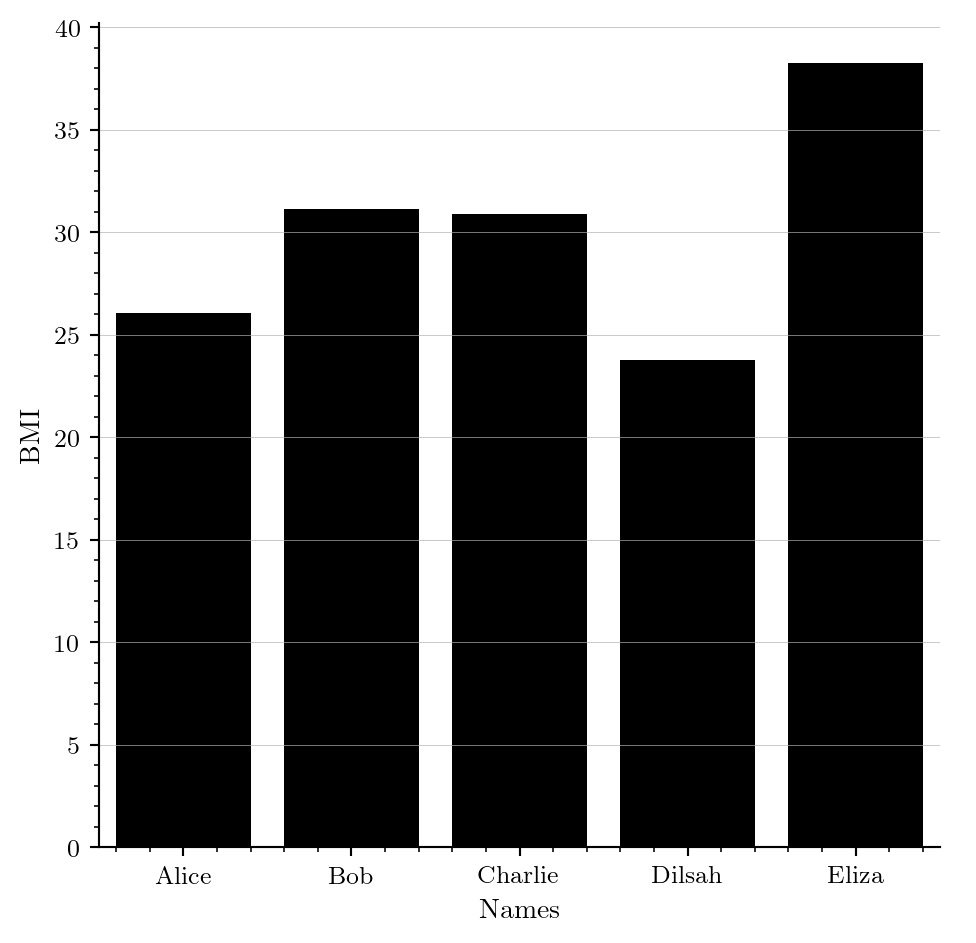
df

Part 2: Visualisation

To visualise the data, we can use the seaborn module, with the function sns.catplot( ... ). Inside the function, we’ll need to specify the x and y values, and if we specifically want a bar plot, kind as well. Use the help() documentation to see if you can visualise the data we just created. See if you can produce something like the following plot:

You’ll need to start with

sns.catplot(data = df, x = ...)

Hint: You only need to use the data =, x =, y = and kind = parameters, so try figure out what they require!

Solution

The plot above is produced with the code

# Visualise
sns.catplot(data = df, x = "Names", y = "BMI", kind = "bar")

Conclusion and saving your work

Save your script as normal. By default, variables are not saved, which is another reason why working with a script is important: you can execute the whole script in one go to get everything back. When you next open the folder in Positron, simply re-run the script to get back to the same state.

Summary

Today we looked at a lot of Python features, so don’t worry if they haven’t all sunk in. Programming is best learned through practice, so keep at it! Here’s a rundown of the concepts we covered

Concept	Desctiption
The console vs scripts	The console is our window into the computer, this is where we send code directly to the computer. Scripts are files which we can write, edit, store and run code, that’s where you’ll write most of your Python.
Variables	Variables are the nouns of programming, this is where we store information, the objects and things of our coding. They come in different types like integers, strings and lists.
Indexing	In order to access elements of a sequence variable, like a list, we need to index, e.g. `myList[2]`. Python counts from 0.
Functions	Functions are the verbs of programming, they perform actions on our variables. Call the function by name and put inputs inside parentheses, e.g. `round(2.5)`
Help	Running `help( ... )` will reveal the help documentation about a function or type.
Conditionals	`if`, `elif` and `else` statements allow us to run code if certain conditions are true, and skip it otherwise.
Loops	`while` loops will repeatedly run code until a condition is no longer true, and `for` loops will iterate through a variable
Packages	We can bring external code into our environment with `import ...`. This is how we use packages, an essential for Python. Don’t forget to install the package first!

Next session

Thanks for completing this introductory session to Python! You’re now ready for our next session, Managing Data, which looks at using the pandas package in greater depth.

Before you go, don’t forget to check out the Python User Group, a gathering of Python users at UQ.

Finally, if you need any support or have any other questions, shoot us an email at training@library.uq.edu.au.

Setup

Introducing Python and Positron

Maths

Variables

Numbers

Booleans

Sequences

Indexing

Scripts and folders

Functions

Operators

General

Mathematical

Comparison

Finding help

Activity 1

Packages

Built-in packages

Naming

Common external packages

An example: numpy

Activity 2

Part 1: Modifying the data

Part 2: Visualisation

Conclusion and saving your work

Summary

Next session

An example: `numpy`