import pandas as pdPython Training (2 of 4): Managing Data
NoteRecent update: Positron
These materials have recently been updated to reflect our shift from Spyder to the Positron IDE.
Positron looks and feels like VS Code with the data science features of RStudio and Spyder.
The Python content remains unchanged.
In this second workshop we will cover
- Examining / exploring data
- Filtering rows and columns
- Basic descriptive statistics
- Adding new columns
- Group bys and summary tables
This hands-on course – directed at intermediate users – looks at using the pandas module to transform and visualise tabular data.
Setting up
Scripts and folders
Recall that we typically write code in scripts and store them in a folder. We’ll do the same here.
- Create / open a folder. If you made one last week, feel free to continue working there. Otherwise, create a new folder for your work and open it with
File > Open folder.... - Create a new script with
New > New file...and choose “Python file” - Save the file to give it a name (e.g.
processing.py)
Introducing pandas
Pandas is a Python module that introduces dataframes to Python. It gives us the tools we need to clean and transform data with Python.
To be able to use the functions included in pandas, we have to first import it:
pd is the usual nickname for the pandas module.
TipInstalling
pandas
If pandas is not installed, you will get an error like No module named 'pandas'.
In Positron, for non-conda users (not using Anaconda), run
%pip install pandasin the console (drop the % if using the terminal). You should restart your Python console before trying to import again.
For (Ana)conda users, replace pip with conda.
The DataFrame object
Pandas is built upon one key feature: the DataFrame class. In Python we have different built-in types, like int for integers and string for characters. Pandas introduces a new type, DataFrame, which stores data like a spreadsheet.
Setting up the workspace
To make life easy, we should set up our workspace well.
- Open your folder using your file explorer, and create a new folder called “data” if you haven’t got one already.
- Download the data for today’s session
- Move the file into your new “data” folder
- Open the explorer pane and check that you see two objects:
- The file “processing.py”
- The folder “data” with your data file(s) inside.
Importing data
Pandas offers a simple way to access data with its read.csv() function. We’ll save it into the variable df_raw:
df_raw = pd.read_csv("data/Players2024.csv")You can also provide a URL instead of a file path!
Aside - File Paths and backslashes
Just a quick detour to discuss file paths of which there are two types: absolute and relative
Absolute
Absolute file paths always start at the “top” of your file system, e.g. one of the drives (like C:) for Windows users, so they are never ambiguous. It’s like providing your full street address from country to street number.
C:/Users/my_username/research/data/really_important_secret_data.csvRelative
Relative file paths start from your current working directory, which is usually folder opened by Positron. For files in my current folder, I just provide their name - like referring to another house on your street as “number 7”. Let’s assume we’re in the “research” folder.
file_in_my_current_folder.csvWe can go to down folders from our current location:
data/really_important_secret_data.csvAnd we can go up folders from our current location
../../this_file_is_two_levels_up.csvOr a combination of the two (e.g. up one, then down into a different folder)
../not_research/this_file_is_not_research.csvWhat matters is that the relative reference depends on where your code is and will break if you move the script!
Backslashes
One last note: Windows uses backslashes for their file paths
C:\Users\...But Python uses backslashes as an escape character. For example, "\n" is a newline, "\u1234" is the unicode character U+1234 and confusingly "\\" is a single backslash. The easist way to get around this is by prefixing R to all strings: this makes them raw.
windows_url = R"C:\\Users\..."Initial look at the data
Let’s get back to data.
We can investigate the size of the data thanks to the shape attribute attached to all pandas dataframes:
df_raw.shape(5935, 7)The dataset contains dozens of columns. What are their names?
df_raw.columnsIndex(['name', 'birth_date', 'height_cm', 'positions', 'nationality', 'age',
'club'],
dtype='object')Let’s subset our data to focus on a handful of variables.
Creating a backup
Data analysis in Python is safe because our variables are copies of the data - we aren’t actually changing the files until we explicitly overwrite them. However, Python also has no undo, so if I delete something in my analysis, I can’t get it back - I have to start all over again.
One way to mitigate this issue is by making a copy of the data
df = df_raw.copy()Now we have two variables: df is what we’ll use, and df_raw stores the raw data. If we ever need to restart, we can simply run df = df_raw.copy().
Accessing and Filtering Data
So how do we access our data in Python? We use a type of indexing introduced by pandas, which revolves around using square brackets after the dataframe: df[...].
Accessing columns
To access a column, index with its name: df["column_name"]. For example,
df["name"]0 James Milner
1 Anastasios Tsokanis
2 Jonas Hofmann
3 Pepe Reina
4 Lionel Carole
...
5930 Oleksandr Pshenychnyuk
5931 Alex Marques
5932 Tomás Silva
5933 Fábio Sambú
5934 Hakim Sulemana
Name: name, Length: 5935, dtype: objectreturns the “name” column. We can access multiple by providing a list of names
# Save the names in a list and then index
column_names = ["name", "club"]
df[column_names]

# This is equivalent to
df[["name", "club"]]| name | club | |
|---|---|---|
| 0 | James Milner | Brighton and Hove Albion Football Club |
| 1 | Anastasios Tsokanis | Volou Neos Podosferikos Syllogos |
| 2 | Jonas Hofmann | Bayer 04 Leverkusen Fußball |
| 3 | Pepe Reina | Calcio Como |
| 4 | Lionel Carole | Kayserispor Kulübü |
| ... | ... | ... |
| 5930 | Oleksandr Pshenychnyuk | ZAO FK Chornomorets Odessa |
| 5931 | Alex Marques | Boavista Futebol Clube |
| 5932 | Tomás Silva | Boavista Futebol Clube |
| 5933 | Fábio Sambú | Boavista Futebol Clube |
| 5934 | Hakim Sulemana | Randers Fodbold Club |
5935 rows × 2 columns
If we want to do anything with it (like statistics or visualisation), it’s worth saving the column(s) as a new variable
df_subset = df[["name", "club"]]Accessing rows
There’s a few ways to access rows. The easiest is by slicing, df[start_row : end_row]. For example, if you want rows 5 to 10,
df[5 : 10]| name | birth_date | height_cm | positions | nationality | age | club | |
|---|---|---|---|---|---|---|---|
| 5 | Ludovic Butelle | 1983-04-03 | 188.0 | Goalkeeper | France | 41 | Stade de Reims |
| 6 | Daley Blind | 1990-03-09 | 180.0 | Defender | Netherlands | 34 | Girona Fútbol Club S. A. D. |
| 7 | Craig Gordon | 1982-12-31 | 193.0 | Goalkeeper | Scotland | 41 | Heart of Midlothian Football Club |
| 8 | Dimitrios Sotiriou | 1987-09-13 | 185.0 | Goalkeeper | Greece | 37 | Omilos Filathlon Irakliou FC |
| 9 | Alessio Cragno | 1994-06-28 | 184.0 | Goalkeeper | Italy | 30 | Associazione Calcio Monza |
Note that the end row is not included
If you want to access a single row, we need to use df.loc[] or df.iloc[]. These are the go-to methods for accessing data if the above indexing isn’t sufficient.
df.loc[]accesses rows by label (defaults to row number but could be anything)df.iloc[]accesses rows by row number exclusively
By default they line up, so
df.loc[5]
df.iloc[5]
name Ludovic Butelle
birth_date 1983-04-03
height_cm 188.0
positions Goalkeeper
nationality France
age 41
club Stade de Reims
Name: 5, dtype: objectare often (but not always) the same.
Finally, we can filter specific rows by a condition on one of the variables, e.g. only rows where variable \(\text{age} > 25\).
df[df["age"] > 25]
# Or any other condition| name | birth_date | height_cm | positions | nationality | age | club | |
|---|---|---|---|---|---|---|---|
| 0 | James Milner | 1986-01-04 | 175.0 | Midfield | England | 38 | Brighton and Hove Albion Football Club |
| 1 | Anastasios Tsokanis | 1991-05-02 | 176.0 | Midfield | Greece | 33 | Volou Neos Podosferikos Syllogos |
| 2 | Jonas Hofmann | 1992-07-14 | 176.0 | Midfield | Germany | 32 | Bayer 04 Leverkusen Fußball |
| 3 | Pepe Reina | 1982-08-31 | 188.0 | Goalkeeper | Spain | 42 | Calcio Como |
| 4 | Lionel Carole | 1991-04-12 | 180.0 | Defender | France | 33 | Kayserispor Kulübü |
| ... | ... | ... | ... | ... | ... | ... | ... |
| 5155 | Leo Scienza | 1998-09-13 | 175.0 | Attack | Brazil | 26 | 1. Fußballclub Heidenheim 1846 |
| 5236 | Mohamed Brahimi | 1998-09-17 | 181.0 | Attack | France | 26 | FK Fakel Voronezh |
| 5287 | Nicolás Marotta | 1996-12-23 | 186.0 | Defender | Argentina | 27 | Athens Kallithea Football Club |
| 5471 | Daniel Sosah | 1998-09-21 | 179.0 | Attack | Niger | 26 | FK Kryvbas Kryvyi Rig |
| 5478 | Egas Cacintura | 1997-10-29 | 174.0 | Midfield | Angola | 26 | Dinamo Makhachkala |
2757 rows × 7 columns
As with the column case, it’s useful to save this as a variable
df_filtered = df[df["age"] > 15]Basic statistics
How might we perform some basic statistics on our data?
To check what kind of data each column is stored as, we can use the dtypes attribute:
df.dtypesname object
birth_date object
height_cm float64
positions object
nationality object
age int64
club object
dtype: objectIn general, pandas will bring in numbers with
float64and non-numeric data withobject.
The describe() method is useful for descriptive statistics about our numerical columns:
df.describe()| height_cm | age | |
|---|---|---|
| count | 5935.000000 | 5935.000000 |
| mean | 182.986352 | 25.501769 |
| std | 7.478313 | 4.455595 |
| min | 17.000000 | 15.000000 |
| 25% | 178.000000 | 22.000000 |
| 50% | 183.000000 | 25.000000 |
| 75% | 188.000000 | 29.000000 |
| max | 206.000000 | 42.000000 |
However, it will only show the two first ones and two last ones. We can focus on a specific column instead, for example one that was hidden previously:
df["age"].describe()count 5935.000000
mean 25.501769
std 4.455595
min 15.000000
25% 22.000000
50% 25.000000
75% 29.000000
max 42.000000
Name: age, dtype: float64Or a categorical column:
df["nationality"].describe()count 5935
unique 135
top Spain
freq 402
Name: nationality, dtype: objectFor a categorical column, the information shown is different: for example, how many unique values there are, and what the most common value is.
What if you want specific statistics about a particular column? Usually there are methods available:
# Applicable to all columns
df["nationality"].count()
df["nationality"].unique()

# For numeric columns only
df["height_cm"].min()
df["height_cm"].max()
df["height_cm"].mean()
df["height_cm"].median()
df["height_cm"].std()
# ...np.float64(7.478312588515905)We can use these methods to filter our data. For example, the row which has the maximum value of variable \(x\) is
x_max = df["height_cm"].max()
df[df["height_cm"] == x_max]

# Or in one line
df[df["height_cm"] == df["height_cm"].max()]| name | birth_date | height_cm | positions | nationality | age | club | |
|---|---|---|---|---|---|---|---|
| 4179 | Kevin Gadellaa | 2003-04-08 | 206.0 | Goalkeeper | Netherlands | 21 | Football Club Utrecht |
| 4810 | Isaak Touré | 2003-03-28 | 206.0 | Defender | France | 21 | Udinese Calcio |
| 5565 | Denys Tvardovskyi | 2003-06-13 | 206.0 | Goalkeeper | Ukraine | 21 | FC Shakhtar Donetsk |
Activity 1
Run the following lines:
print(df["height_cm"].min())
print(df["positions"].unique())
17.0
['Midfield' 'Goalkeeper' 'Defender' 'Attack' 'Missing']Notice anything odd? There’s some dubious data - remove the dodgy entries.
Hint: Nobody is 17cm tall, and we don’t want to keep anyone with the “Missing” position either
NoteSolution
# Remove rows with unreasonable heights
df = df[df["height_cm"] > 100]

# Remove the rows with position = "Missing"
df = df[df["positions"] != "Missing"]
If that was too quick try to reduce your dataset to \(\le 3\) variables (columns) and \(\le 100\) rows using conditions by filtering down to a particular subset of your data. Make sure you keep the age and height_cm columns.
Adding and removing columns
Sometimes we need to add new columns. It’s the same process as overwriting existing columns - let’s make a new column called “zeroes” where every row is 0
df["zeroes"] = 0We can also send in a column, for example
df["copy_of_names"] = df["name"]Perhaps most usefully, we can manipulate the column we send in. For example, the deviation from the mean \[|\bar{x} - x_i|\] can be computed for each row’s height:
col_x = df["height_cm"]
avg_x = df["height_cm"].mean()

df["deviation_from_mean_height"] = abs(col_x - avg_x)

# Or all together on one line,
df["deviation_from_mean_height"] = abs(df["height_cm"] - df["height_cm"].mean())
where abs(...) takes the absolute value
Notice that we subtracted a value from a column. We can also perform mathematics with multiple columns:
df["product"] = df["age"]*df["height_cm"]Let’s remove these new columns that we don’t need with the method df.drop(columns = [...]):
df = df.drop(columns = ["zeroes", "copy_of_names", "deviation_from_mean_height", "product"])Summaries
After cleaning up our data, we need to analyse it. This usually involves some kind of aggregation. For example, what is the average \(x\) per year? requires aggregating over variable \(x\) for each year.
First, we need to group by a specific variable
gb = df.groupby("age")This thing in itself is a pretty abstract Python object, best thought of as a dataframe where we’ve identified a grouping variable.
Next, we need to apply some aggregation to it (the groupby tells it to do it for each year)
avg_height_by_age = gb["height_cm"].agg("mean")Of course, we could have done this in one line:
avg_height_by_age = df.groupby("age")["height_cm"].agg("mean")This is a really useful tool, because now we have something we can visualise. As the next session will show us, the visualisation tools generally just take in numbers and turn them into dots. We need to do the stats beforehand.
As a taster, try running
avg_height_by_age.plot()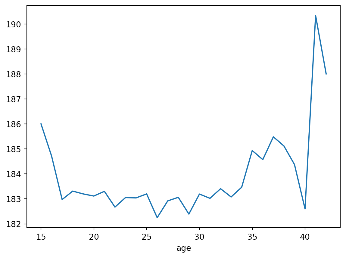
Exporting results
The last step in the process is saving the data. Let’s say we want to take that final dataframe and export it to a csv. That’s what the df.to_csv() method is for
avg_height_by_age.to_csv("data/avg_height_by_age.csv")This will save the dataframe to a .csv file and place it in the data folder.
Activity 2
Now that you’ve explored our “Players” dataset, why not try something larger? Download the gapminder dataset and explore. Try to use the following three techniques:
- Filter the data by a condition
- Aggregate over a particular variable
- Visualise your result
For step 3., you’ll either want to reduce your data to two columns and use .plot(), or specify your axes with .plot(x = "x_variable", y = "y_variable").
NoteSolution
One possible solution with aggregation is
# Import the data
gapminder = pd.read_csv("data/gapminder.csv")

# Select specific columns
subset = gapminder[["continent", "year", "pop"]]

# Max pop per continent of all time
continents = subset.groupby("continent").agg("max")

continents.plot(y = "pop", kind = "bar")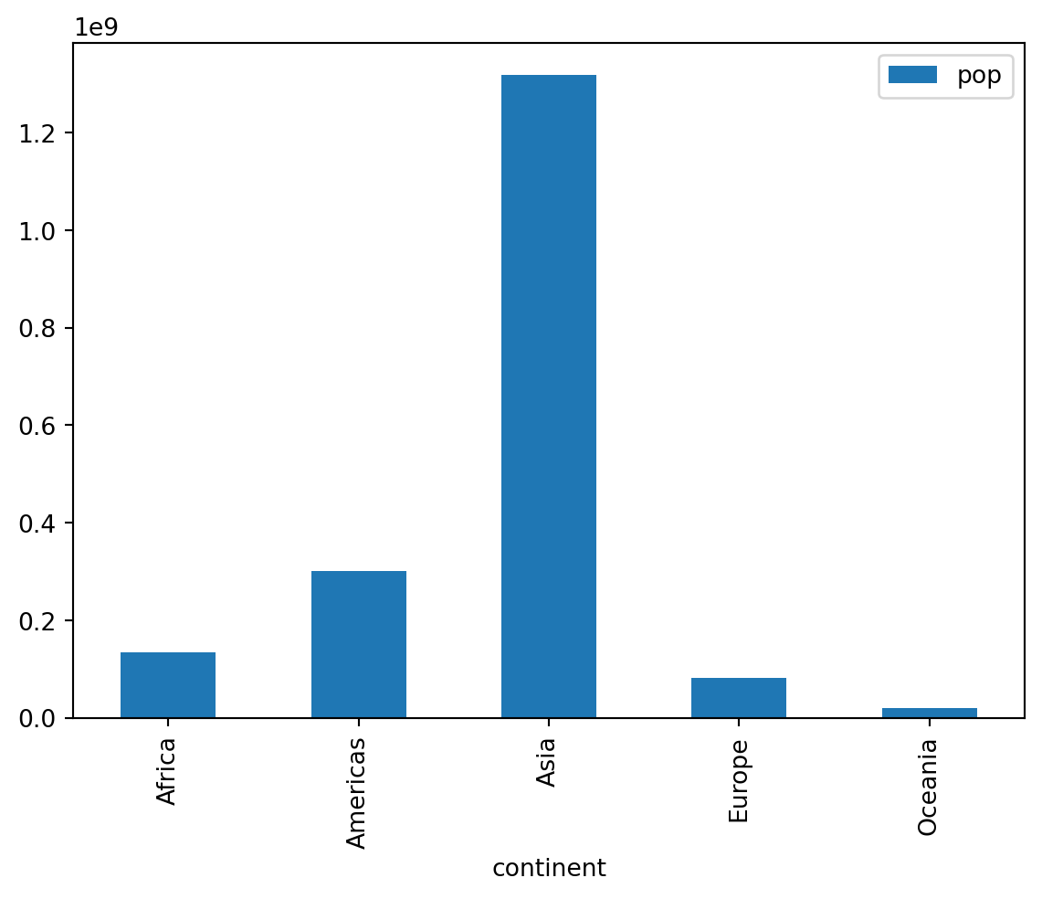
Conclusion
Today we looked at a lot of Python features, so don’t worry if they haven’t all sunk in. Programming is best learned through practice, so keep at it! Here’s a rundown of the concepts we covered
| Concept | Desctiption |
|---|---|
| Importing data | The pandas package provides the pd.read_... functions to import data, like pd.read_csv(). Save it in a variable. |
| Accessing and filtering rows and columns | Use square brackets for basic accessing and filtering, e.g. df["column_a"] or df[df["column_b"] > 5]. |
| Basic statistics | A number of basic statistical functions can be applied to columns, e.g. df["column_a"].max(). |
| Adding and removing columns | Add columns by pretending they’re already there and assigning into them, df["new_column"] = ..., and remove them with df = df.drop(columns = [...]). |
| Summaries and grouping | Use df.groupby("variable_a").agg("statistic_b") to aggregate over your data. |
| Exporting | Use df.to_csv("file_path") to export your data |
Next session
Thanks for completing this introductory session to Python! You’re now ready for our next session, introductory visualisation, which looks at using the seaborn package for making visualisations.
Before you go, don’t forget to check out the Python User Group, a gathering of Python users at UQ.
Finally, if you need any support or have any other questions, shoot us an email at training@library.uq.edu.au.
Resources
- Official pandas documentation
- More visualisation modules:
- Our compilation of useful Python links