R dplyr: preparing data for analysis

Author

UQ Library

Published

April 14, 2025

What are we going to learn?

In this hands-on session, you will use R, RStudio and the dplyr package to transform your data.

Specifically, you will learn how to explore, filter, reorganise and process a table of data with the following verbs:

select(): pick variables
filter(): pick observations
arrange(): reorder observations
mutate(): create new variables
summarise(): collapse to a single summary
group_by(): change the scope of function

Keep in mind

Everything we write today will be saved in your project. Please remember to save it in your H drive or USB if you are using a Library computer.
R is case sensitive: it will tell the difference between uppercase and lowercase.
Respect the naming rules for objects (no spaces, does not start with a number…)

Help

For any dataset or function doubts that you might have, don’t forget the three ways of getting help in RStudio:

the shortcut command: ?functionname
the help function: help(functionname)
the keyboard shortcut: press F1 after writing a function name

Open RStudio

If you are using your own laptop please open RStudio
- If you need them, we have installation instructions
Make sure you have a working internet connection
On Library computers (the first time takes about 10 min.):
- Log in with your UQ credentials (student account if you have two)
- Make sure you have a working internet connection
- Go to search at bottom left corner (magnifiying glass)
- Open the ZENworks application
- Look for RStudio
- Double click on RStudio which will install both R and RStudio

Setting up

Install the dplyr package

If you don’t have it already, you can install dplyr with the command: install.packages("dplyr")

At home, you can install the whole “tidyverse”, a meta-package useful for data science: install.packages("tidyverse")

New project

Click the “File” menu button (top left corner), then “New Project”
Click “New Directory”
Click “New Project” (“Empty project” if you have an older version of RStudio)
In “Directory name”, type the name of your project, e.g. “dplyr_intro”
Select the folder where to locate your project: for example, the Documents/RProjects folder, which you can create if it doesn’t exist yet.
Click the “Create Project” button

Create a script

We will use a script to write code more comfortably.

Menu: Top left corner, click the green “plus” symbol, or press the shortcut (for Windows/Linux) Ctrl+Shift+N or (for Mac) Cmd+Shift+N. This will open an “Untitled1” file.
Go to “File > Save” or press (for Windows/Linux) Ctrl+S or (for Mac) Cmd+S. This will ask where you want to save your file and the name of the new file.
Call your file “process.R”

Introducing our data

Challenge 1 – import data

Let’s import and explore our data.

read the data into an object called “gapminder”, using read.csv():

gapminder <- read.csv("https://raw.githubusercontent.com/resbaz/r-novice-gapminder-files/master/data/gapminder-FiveYearData.csv")

Remember you can use Ctrl+shift to execute a command from the script.

Explore the gapminder dataset using dim() and str()

How can we get the dataframe’s variable names? There are two ways: names(gapminder) returns the names regardless of the object type, such as list, vector, data.frame etc., whereas colnames(gapminder) returns the variable names for matrix-like objects, such as matrices, dataframes…

To return one specific column in the dataframe, you can use the dollar syntax: gapminder$year. For example, try these:

class(gapminder$country) # what kind of data?

[1] "character"

range(gapminder$year) # what is the time range?

[1] 1952 2007

Basic dplyr verbs

The R package dplyr was developed by Hadley Wickham for data manipulation.

The book R for Data Science introduces the package as follows:

You are going to learn the five key dplyr functions that allow you to solve the vast majority of your data manipulation challenges:

Pick variables by their names with select()

Pick observations by their values with filter()

Reorder the rows with arrange()

Create new variables with functions of existing variables with mutate()

Collapse many values down to a single summary with summarise()

These can all be used in conjunction with group_by() which changes the scope of each function from operating on the entire dataset to operating on it group-by-group. These six functions provide the main verbs for a language of data manipulation.

To use the verbs to their full extent, we will need pipes and logical operators, which we will introduce as we go.

Let’s load the dplyr package to access its functions:

library(dplyr)


Attaching package: 'dplyr'

The following objects are masked from 'package:stats':

    filter, lag

The following objects are masked from 'package:base':

    intersect, setdiff, setequal, union

You only need to install a package once (with install.packages()), but you need to reload it every time you start a new R session (with library()).

1. Pick variables with `select()`

select() allows us to pick variables (i.e. columns) from the dataset. For example, to only keep the data about year, country and GDP per capita:

gap_small <- select(gapminder, year, country, gdpPercap)

The first argument refers to the dataframe that is being transformed, and the following arguments are the columns you want to keep. Notice that it keeps the order you specified?

You can also rename columns in the same command:

gap_small <- select(gapminder, year, country, gdpPerPerson = gdpPercap)

If you have many variables but only want to remove a small number, it might be better to deselect instead of selecting. You can do that by using the - character in front of a variable name:

names(select(gapminder, -continent))

[1] "country"   "year"      "pop"       "lifeExp"   "gdpPercap"

There are also a lot of helper functions to select columns according to a logic. For example, to only keep the columns that have “a” in their names:

names(select(gapminder, contains("a")))

[1] "year"      "gdpPercap"

2. Pick observations with `filter()`

The filter() function allows use to pick observations depending on one or several conditions. But to be able to define these conditions, we need to learn about logical operators.

Logical operators allow us to compare things. Here are some of the most important ones:

==: equal
!=: different or not equal
>: greater than
<: smaller than
>=: greater or equal
<=: smaller or equal

Remember: = is used to pass on a value to an argument, whereas == is used to check for equality. Using = instead of == for a logical statment is one of the most common errors and R will give you a reminder in the console when this happens.

You can compare any kind of data For example:

1 == 1

[1] TRUE

1 == 2

[1] FALSE

1 != 2

[1] TRUE

1 > 0

[1] TRUE

"money" == "happiness"

[1] FALSE

When R executes these commands, it answers TRUE of FALSE, as if asked a yes/no question. These TRUE and FALSE values are called logical values.

Note that we can compare a single value to many. For example, compare one value to three others:

1 == c(1, 2, 3, 1, 3)

[1]  TRUE FALSE FALSE  TRUE FALSE

This kind of operation results in a logical vector with a logical value for each element. This is exactly what we will use to filter our rows.

For example, to filter the observations for Australia, we can use the following condition:

australia <- filter(gapminder, country == "Australia")
australia

The function compares the value “Australia” to all the values in the country variable, and only keeps the rows that have TRUE as an answer.

Now, let’s filter the rows that have a life expectancy lifeExp greater than 81 years:

life81 <- filter(gapminder, lifeExp > 81)
dim(life81)

[1] 7 6

3. Reorder observations with `arrange()`

arrange() will reorder our rows according to a variable, by default in ascending order:

arrange(life81, lifeExp)

If we want to have a look at the entries with highest life expectancy first, we can use the desc() function (for “descending”):

arrange(life81, desc(lifeExp))

We could also use the - shortcut, which only works for numerical data:

arrange(life81, -lifeExp)

The pipe operator

What if we wanted to get that result in one single command, without an intermediate life81 object?

We could nest the commands into each other, the first step as the first argument of the second step:

arrange(filter(gapminder, lifeExp > 81), -lifeExp)

… but this becomes very hard to read, very quickly. (Imagine with 3 steps or more!)

We can make our code more readable and avoid creating useless intermediate objects by piping commands into each other. The pipe operator %>% strings commands together, using the left side’s output as the first argument of the right side function.

For example, this command:

round(1.23, digits = 1)

[1] 1.2

… is equivalent to:

1.23 %>% round(digits = 1)

[1] 1.2

Here’s another example with the filter() verb:

gapminder %>%
  filter(country != "France")

… becomes:

filter(gapminder, country != "France")

To do what we did previously in one single command, using the pipe:

gapminder %>% 
  filter(lifeExp > 81) %>% 
  arrange(-lifeExp)

The pipe operator can be read as “then” and makes the code a lot more readable than when nesting functions into each other, and avoids the creation of several intermediate objects. It is also easier to troubleshoot as it makes it easy to execute the pipeline step by step.

From now on, we’ll use the pipe syntax as a default.

Note that this material uses the magrittr pipe. The magrittr package is the one that introduced the pipe operator to the R world, and dplyr automatically imports this useful operator when it is loaded. However, the pipe being such a widespread and popular concept in programming and data science, it ended up making it into Base R (the “native” pipe) in 2021 with the release of R 4.1, using a different operator: |>. You can switch your pipe shortcut to the native pipe in Tools > Global options > Code > Use native pipe operator.

Challenge 2 – a tiny dataset

Only keep the 2002 life expectancy observation for Eritrea and remove the superfluous variables.

eritrea_2002 <- gapminder %>%
    select(year, country, lifeExp) %>%
    filter(country == "Eritrea", year == 2002)

4. Create new variables with `mutate()`

Have a look at what the verb mutate() can do with ?mutate.

Let’s see what the two following variables can be used for:

gapminder %>%
    select(gdpPercap, pop)

How do you think we could combine them to add something new to our dataset?

Challenge 3 – mutate the GDP

Use mutate() to create a gdp variable.

Name your new dataset gap_gdp. When finished, dim(gap_gdp) should result in 1704 7.

Hint: use the * operator within mutate().

gap_gdp <- gapminder %>%
    mutate(gdp = gdpPercap * pop)
dim(gap_gdp)

[1] 1704    7

head(gap_gdp)

You can reuse a variable computed by ‘mutate()’ straight away. For example, we also want a more readable version of our new variable, in billion dollars:

gap_gdp <- gapminder %>%
    mutate(gdp = gdpPercap * pop,
           gdpBil = gdp / 1e9)

5. Collapse to a single value with `summarise()`

summarise() collapses many values down to a single summary. For example, to find the mean life expectancy for the whole dataset:

gapminder %>%
  summarise(meanLE = mean(lifeExp))

However, a single-value summary is not particularly interesting. summarise() becomes more powerful when used with group_by().

6. Change the scope with `group_by()`

group_by() changes the scope of the following function(s) from operating on the entire dataset to operating on it group-by-group.

See the effect of the grouping step:

gapminder %>%
    group_by(continent)

The data in the cells is the same, the size of the object is the same. However, the dataframe was converted to a tibble, because a dataframe is not capable of storing grouping information.

Using the group_by() function before summarising makes things more interesting. Let’s re-run the previous command, with the intermediate grouping step:

gapminder %>%
  group_by(continent) %>% 
  summarise(meanLE = mean(lifeExp))

We now have the summary computed for each continent.

Similarly, to find out the total population per continent in 2007, we can do the following:

gapminder %>% 
    filter(year == 2007) %>%
    group_by(continent) %>%
    summarise(pop = sum(pop))

Challenge 4 – max life expectancy per country

Group by country, and find out the maximum life expectancy ever recorded for each one.

Hint: ?max

gapminder %>% 
    group_by(country) %>%
    summarise(maxLE = max(lifeExp))

More examples

Another example of a summary, with a the starwars data set that dplyr provides:

Grouping by species, summarise the number of characters per species and find the mean mass. Only for species groups with more than 1 character.

starwars %>%
  group_by(species) %>%
  summarise(
    n = n(), # this counts the number of rows in each group
    mass = mean(mass, na.rm = TRUE)
  ) %>%
  filter(n > 1) # the mean of a single value is not worth reporting

An example of data manipulation and data visualisation in the same command with gapminder:

Summarise the gapminder population data into total population per continent per year and plot coloured by continent.

# increase in population per continent
library(ggplot2)
gapminder %>% 
  group_by(continent, year) %>% 
  summarise(pop = sum(pop)) %>% 
  ggplot(aes(x = year,
             y = pop,
             colour = continent)) +
  geom_line()

`summarise()` has grouped output by 'continent'. You can override using the
`.groups` argument.

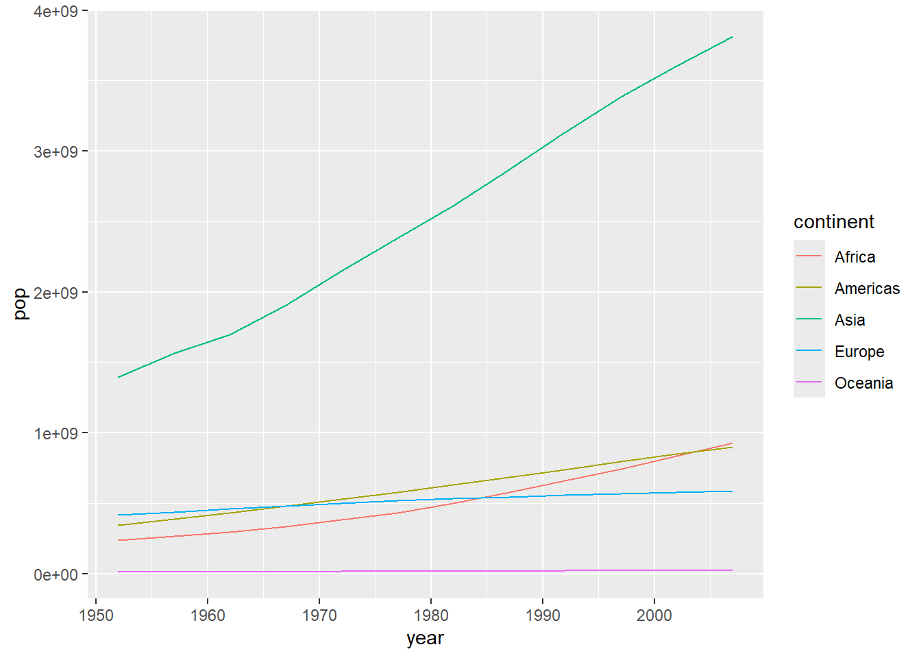
And another example, using using our gapminder dataset:

Let’s say we want to calulate the variation (range) in life expectancy per country and plot the top and bottom 10 countries?

gapminder %>% 
  group_by(country) %>% 
  summarise(maxLifeExp = max(lifeExp),
            minLifeExp = min(lifeExp)) %>% 
  mutate(dif = maxLifeExp - minLifeExp) %>%  # new col with difference betwen max/min lifeExp
  arrange(desc(dif)) %>%  # arrange by dif, descending order for the next step
  slice(1:10, (nrow(.)-10):nrow(.)) %>%  # slice top 10 rows and bottom 10 rows
  ggplot(aes(x = reorder(country, dif), y = dif)) +
  geom_col() +
  coord_flip() + # flip the x and y axis for a horizontal bar chart
  labs(x = "Country",
       y = "Difference in Life Expectancy") + # prettier labels for axes (which have been flipped) 
  annotate("segment", x = 11.5, xend = 21.5, y = 39, yend = 39, colour = "purple", size=1, alpha=0.6) +
  annotate("segment", x = 0.5, xend = 11, y = 39, yend = 39, colour = "green", size=1, alpha=0.6) +
    annotate("text", x = c(5, 16), y = c(40, 40), 
           label = c("Smallest 10", "Largest 10") ,
           color="black", size= 5 , angle=90) # add labels to colored lines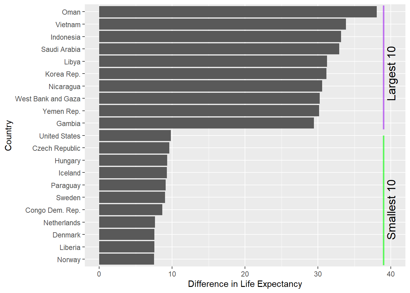

Warning: Using `size` aesthetic for lines was deprecated in ggplot2 3.4.0.
ℹ Please use `linewidth` instead.

Close project

If you want to close RStudio, make sure you save your script first.

You can then close the window, and if your script contains all the steps necessary for your data processing, it is safer to not save your workspace at the prompt. It should only take a second te execute all the commands stored in your script when you re-open your project.