Getting started
You’re welcome to dive in and work as you please, but if you’re feeling at a loss where to begin, follow the scaffold below. Don’t forget to start from our template and look at the examples:
Project scaffold
Step 0: Pick a dataset
We have nine datasets for you to choose from. We recommend saving your data inside your project.
| Dataset | Description | Source |
|---|---|---|
| World populations | A summary of world populations and corresponding statistics | Data from a Tidy Tuesday post on 2014 CIA World Factbook data |
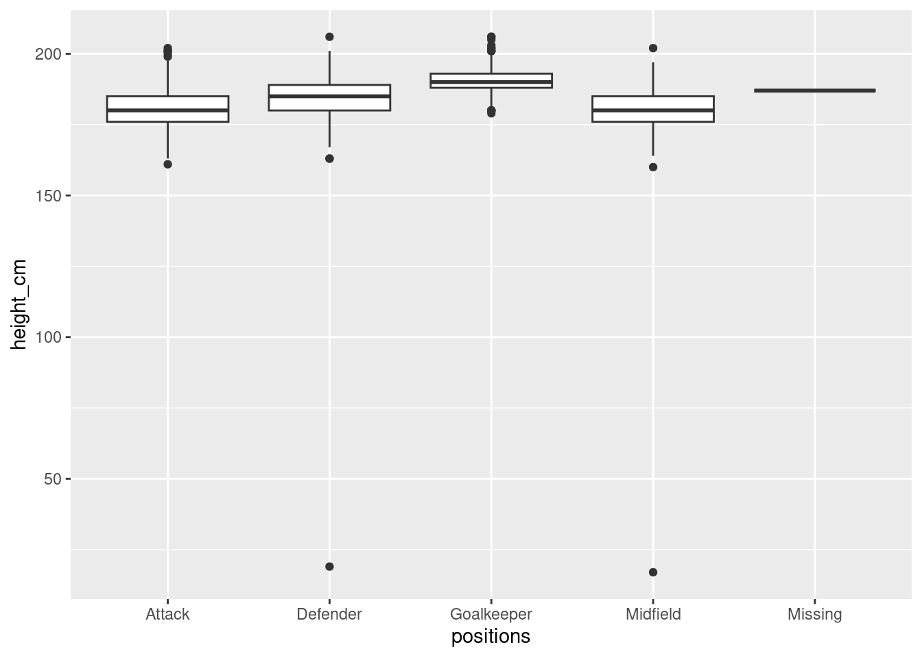
| Soccer players | A summary of approx. 6000 soccer players from 2024 | Data from a Kaggle submission. |
| Coffee survey | A survey of blind coffee tasting results | Data from a Kaggle submission |
| Gapminder | GDP and life expectancy data by country | Data from the Research Bazaar’s R novice tutorial, sourced from Gapminder. |
| Melbourne housing data | A collection of houses for sale in Melbourne. | Data from a Kaggle submission |
| Goodreads books | A summary of books on Goodreads. | Data from a Kaggle submission |
| Queensland hospitals | Queensland emergency department statistics. | Data from the Queensland Government’s Open Data Portal. |
| Queensland fuel prices | Fuel prices by the pump in Queensland | Data from the Queensland Government’s Open Data Portal |
| Aeroplane bird strikes | Aeroplane bird strike incidents fron the 90s | Data from a Tidy Tuesday post sourced from an FAA database |
Remember, to work with data, we should import our useful packages and load the data in.
library(dplyr)
dataset <- read.csv("path_to_data")
import pandas as pd
df = pd.read_csv("data/...")Step 1: Understand the data
The datasets are varied with respect to variable types and content. The first exercise you should complete is a overview of the data. Use the following techniques to do so.
Your goal: identify which variables are discrete (categorical) and which are continuous.
Viewing the data structure
Use the following functions to view your data and the underlying data types.
names(dataset)
str(dataset)
summary(dataset)
df.columns
df.info()
df.describe()Picking out individual columns
To view the contents of particular columns, you can select them via indexing
dataset$column_name
unique(dataset$column_name)
summary(dataset$column_name)
You can also apply other statistics to the column, like max(dataset$column_name).
df["column_name"]
df["column_name"].unique()
df["column_name"].describe()
You can also apply other statistics to the column, like dataset["column_name"].max().
Step 2: Taking a subset
The datasets have lots of observations for lots of variables. To draw meaningful results, it’s often useful to take a subset of those.
Your goal: filter by a condition or group by and aggregate over a particular variable
Filtering
Recall that filtering looks like indexing. If you only want to examine a certain subset of a variable, the following code will isolate that subset
subset = dataset %>% filter(condition)where condition depends on the columns. For example, country == "Australia".
We’ve used the pipe operator %>% here, which is equivalent to filter(datatset, condition).
subset = df[condition]where condition depends on the columns. For example, df["country"] == "Australia".
Grouping
If you want to aggregate over a particular variable you need to group by it. This answers questions like, what is the average \(x\) for every \(y\).
If you want to group by a column and, for each of its values, apply a statistic to all the others,
aggregated <- dataset %>%
  group_by("variable_to_group_by") %>%
  summarise(summary_1 = ..., summary_2 = ..., ...)
The summarise function aggregates by applying some statistic to a particular column for every unique value in the grouping variable. For example, summarise(avg_pop = mean(population)) makes a column in the summary table for the average population of each unique value in "variable_to_group_by".
aggregated = df.groupby("column_to_group_by").agg("statistic")For example, df.groupby("age").agg("max") will calculate the maximum value of every column for every unique age. If you only want to apply aggregation to some columns, we can pick them out,
aggregated = df.groupby("column_to_group_by")["column_to_aggregate"].agg("statistic")By default, df.groupby() makes the grouped column the row names (index). If you want to keep it as a normal column (e.g. for visualisations), you might want to use df.groupby("column", as_index = False)....
Step 3: Visualise the relationship between variables
With your summary dataset, you can now try to visualise your variables.
Your goal: create a visualisation of one to three variables in your summary data.
First, you need to import the appropriate visualisation module
library(ggplot2)We use
import seaborn as snsfor our simple plots and the examples below. You could also use
import matplotlib.pyplot as plt
import plotly.express as px
Next, you’ll need to identify the variables to visualise. If they’re both continuous, you could use a scatter or line plot
Using ggplot, we then specify the data, the mappings and the graphical elements.
ggplot(data = ...,
       mapping = aes(x = ..., y = ..., ...)) +
  geom_...()
Use different graphical elements for different type of variables. Below are a few (non-exhaustive!) options.
If they’re both continuous
geom_line()geom_point()(scatter plot)
If one is categorical
geom_box()geom_bar()(displays the count of each variable)geom_col()(plots \(x\) against \(y\); only have one “number” for each categorical variable - it does not aggregate).
For distributions
geom_hist()
Use different functions and kinds for different variable types. Below are a few (non-exhaustive!) options.
If they’re both continuous
sns.relplot(data = ..., x = ..., y = ..., kind = ..., ...)kind = "scatter"kind = "line"
If one is categorical
sns.catplot(data = ..., x = ..., y = ..., kind = ..., ...)kind = "box"kind = "bar"
For distributions
sns.displot(data = ..., x = ..., kind = ..., ...)kind = "hist"
Step 4: Looking ahead
Now that you’ve performed your first analysis and visualisation of the dataset, use these results to inform your next analysis!
Below you’ll find some general tips which can help. They have dataset-specific tips too, so check them out. Otherwise, feel free to ask if you have any other questions.