Wildlife

26Summer

Author

Nayomi and Julian

Published

January 1, 2026

Introduction

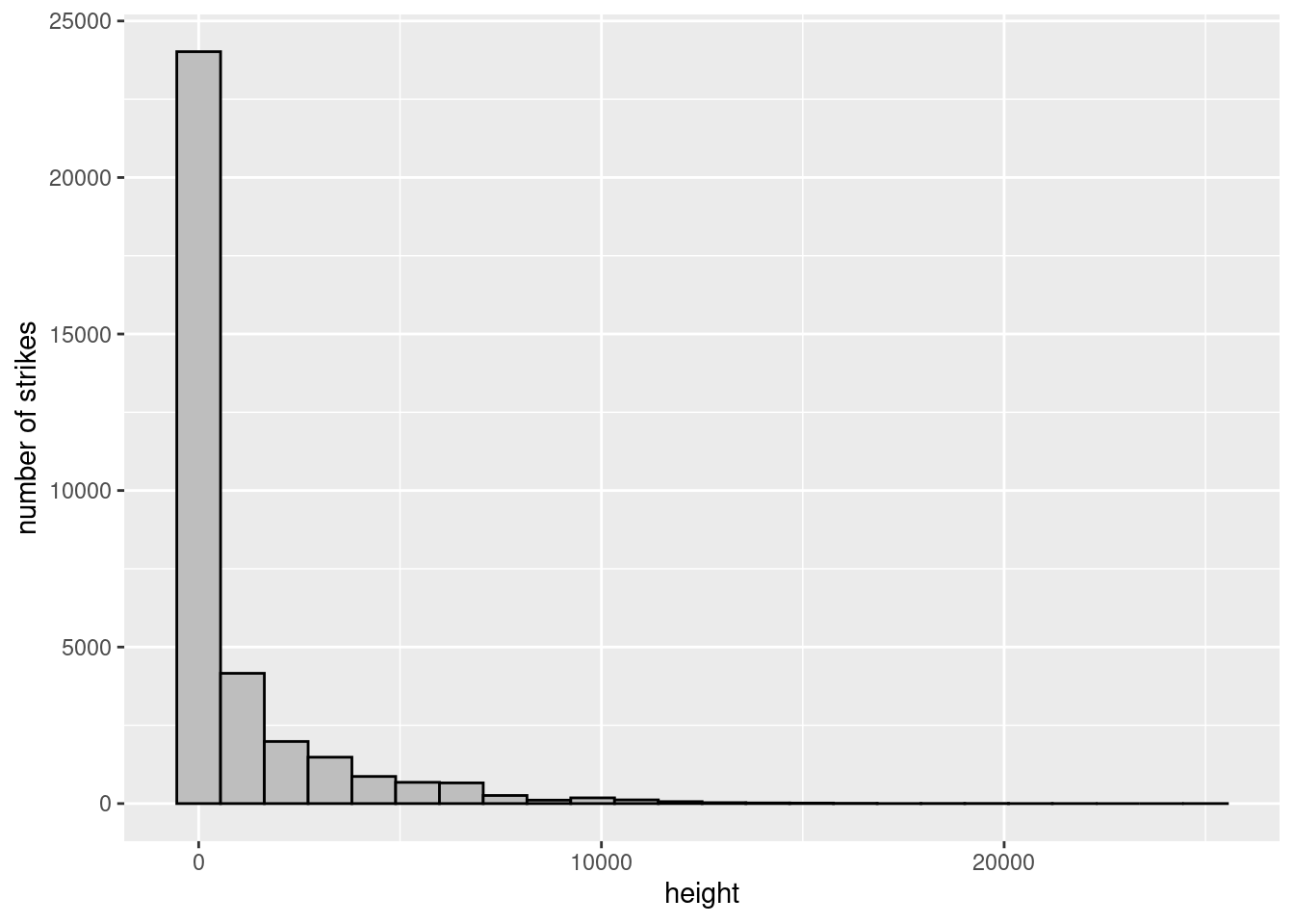
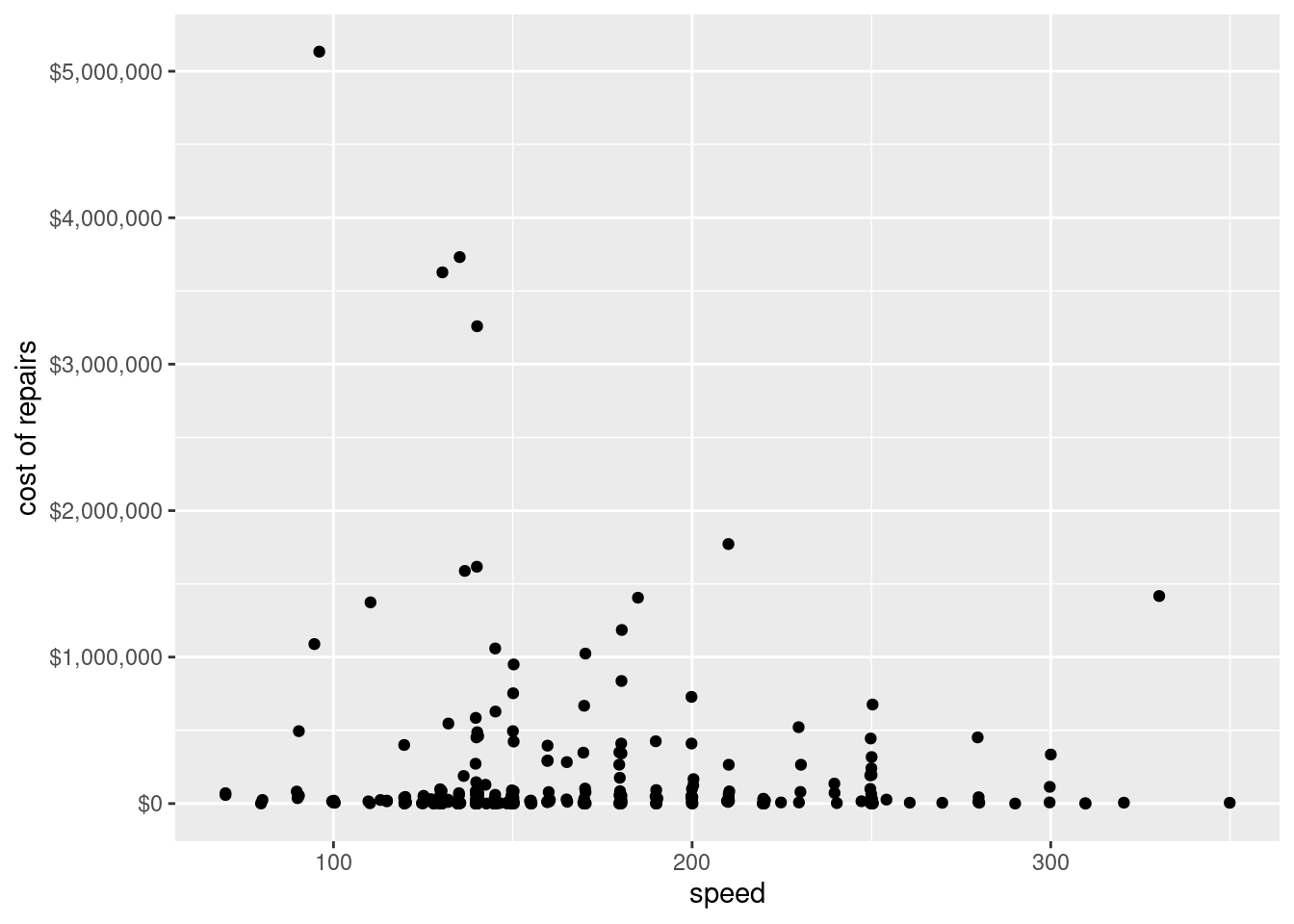
The database we used here contains records of reported wildlife strikes since 1990. this contains self reported strikes from airlines, airports, pilots, and other sources.

Import the data set and install data packages

wildlife_raw <- read.csv('data/wildlife_impacts.csv')
library(dplyr)


Attaching package: 'dplyr'

The following objects are masked from 'package:stats':

    filter, lag

The following objects are masked from 'package:base':

    intersect, setdiff, setequal, union

library(ggplot2)
library(knitr)

This is how the data set looks like

head(wildlife_raw)

         incident_date state airport_id                airport
1 2018-12-31T00:00:00Z    FL       KMIA             MIAMI INTL
2 2018-12-29T00:00:00Z    IN       KIND INDIANAPOLIS INTL ARPT
3 2018-12-29T00:00:00Z   N/A       ZZZZ                UNKNOWN
4 2018-12-27T00:00:00Z   N/A       ZZZZ                UNKNOWN
5 2018-12-27T00:00:00Z   N/A       ZZZZ                UNKNOWN
6 2018-12-27T00:00:00Z    FL       KMIA             MIAMI INTL
           operator     atype type_eng species_id              species damage
1 AMERICAN AIRLINES B-737-800        D      UNKBL Unknown bird - large     M?
2 AMERICAN AIRLINES B-737-800        D          R                 Owls      N
3 AMERICAN AIRLINES   UNKNOWN     <NA>      R2004      Short-eared owl   <NA>
4 AMERICAN AIRLINES B-737-900        D      N5205     Southern lapwing     M?
5 AMERICAN AIRLINES B-737-800        D      J2139         Lesser scaup     M?
6 AMERICAN AIRLINES     A-319        D       UNKB         Unknown bird      N
  num_engs incident_month incident_year time_of_day time height speed
1        2             12          2018         Day 1207    700   200
2        2             12          2018       Night 2355      0    NA
3       NA             12          2018        <NA>   NA     NA    NA
4        2             12          2018        <NA>   NA     NA    NA
5        2             12          2018        <NA>   NA     NA    NA
6        2             12          2018         Day  955     NA    NA
  phase_of_flt        sky precip cost_repairs_infl_adj
1        Climb Some Cloud   None                    NA
2 Landing Roll       <NA>   <NA>                    NA
3         <NA>       <NA>   <NA>                    NA
4         <NA>       <NA>   <NA>                    NA
5         <NA>       <NA>   <NA>                    NA
6     Approach       <NA>   <NA>                    NA

Table1 <- head(wildlife_raw)
kable(Table1)

incident_date	state	airport_id	airport	operator	atype	type_eng	species_id	species	damage	num_engs	incident_month	incident_year	time_of_day	time	height	speed	phase_of_flt	sky	precip	cost_repairs_infl_adj
2018-12-31T00:00:00Z	FL	KMIA	MIAMI INTL	AMERICAN AIRLINES	B-737-800	D	UNKBL	Unknown bird - large	M?	2	12	2018	Day	1207	700	200	Climb	Some Cloud	None	NA
2018-12-29T00:00:00Z	IN	KIND	INDIANAPOLIS INTL ARPT	AMERICAN AIRLINES	B-737-800	D	R	Owls	N	2	12	2018	Night	2355	0	NA	Landing Roll	NA	NA	NA
2018-12-29T00:00:00Z	N/A	ZZZZ	UNKNOWN	AMERICAN AIRLINES	UNKNOWN	NA	R2004	Short-eared owl	NA	NA	12	2018	NA	NA	NA	NA	NA	NA	NA	NA
2018-12-27T00:00:00Z	N/A	ZZZZ	UNKNOWN	AMERICAN AIRLINES	B-737-900	D	N5205	Southern lapwing	M?	2	12	2018	NA	NA	NA	NA	NA	NA	NA	NA
2018-12-27T00:00:00Z	N/A	ZZZZ	UNKNOWN	AMERICAN AIRLINES	B-737-800	D	J2139	Lesser scaup	M?	2	12	2018	NA	NA	NA	NA	NA	NA	NA	NA
2018-12-27T00:00:00Z	FL	KMIA	MIAMI INTL	AMERICAN AIRLINES	A-319	D	UNKB	Unknown bird	N	2	12	2018	Day	955	NA	NA	Approach	NA	NA	NA

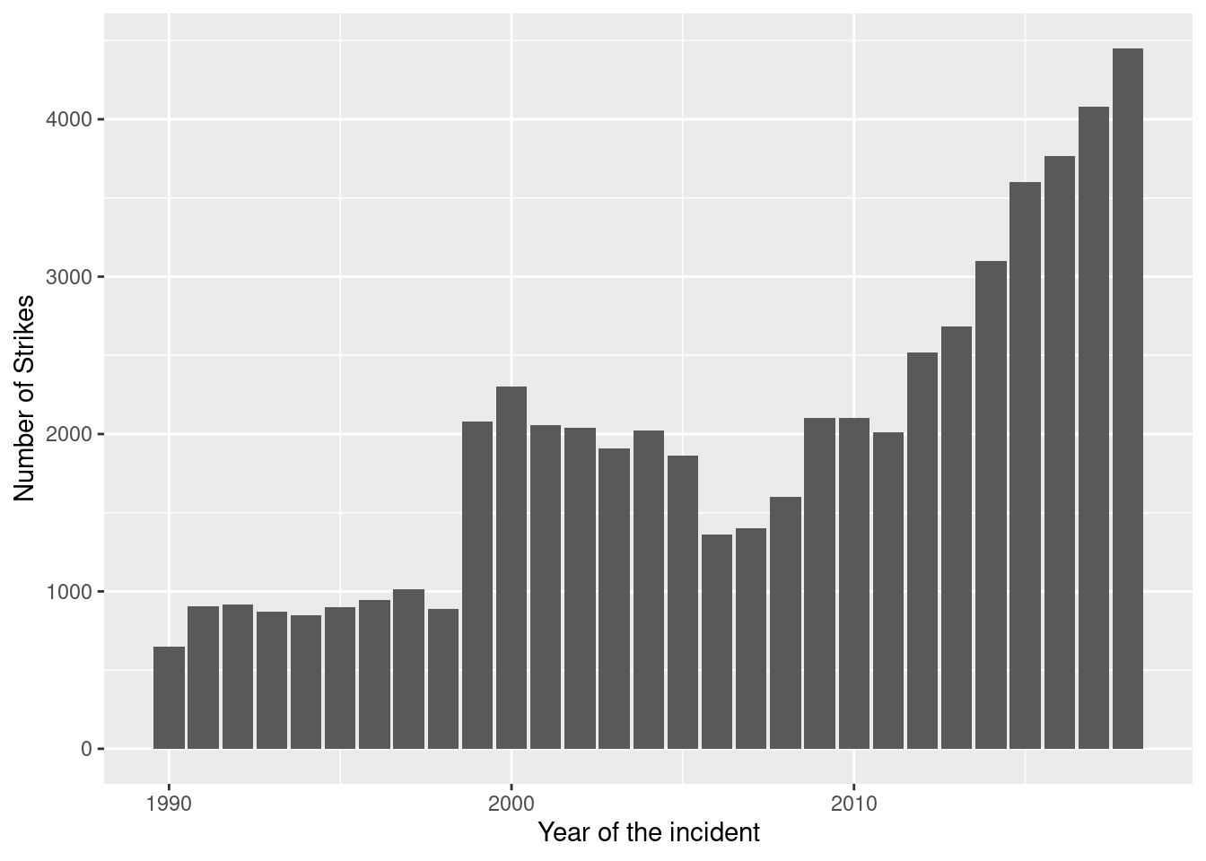
Let’s see the trend over years Is this really increasing over time or proportionately the same???

ggplot(wildlife_raw,
       aes(x=incident_year,))+geom_bar()+labs(x="Year of the incident", y="Number of Strikes")

Data purification

There were a lot of NAs in the data set and treated accordingly.

e.g.

wildlife_cor1 <- wildlife_raw %>% 
  filter(!is.na(speed))
wildlife_cor1 <- wildlife_cor1 %>% 
  filter(!is.na(damage))

Analysis

Differences in strike count according to month of year

ggplot(wildlife_raw,
       aes(x=incident_month, colour=operator))+geom_bar()+
  labs(x="Month", y="Number of Strikes")

Histogram number of strikes at height

wildlife_impacts <- read.csv("data/wildlife_impacts.csv")
wildlife_impacts <- wildlife_impacts %>%
  filter(!is.na(height))
wildlife_impacts <- wildlife_impacts %>%
  filter(!is.na(time_of_day))
ggplot(data = wildlife_impacts,
       aes(x = time_of_day, y = height)) + 
  geom_boxplot(colour = "black", fill = "gray") + 
  labs(x = "time of day", y = "height")

Time of day and strike count

library(ggplot2)
wildlife_impacts <- wildlife_impacts %>%
  filter(!is.na(time_of_day))
ggplot(data = wildlife_impacts,
       aes(x = time_of_day)) + 
         geom_bar(fill = "gray", colour = "black") + 
  labs(x = "time of day", y = "number of strikes")

Histogram of time of day and height of strike

ggplot(data = wildlife_impacts,
       mapping = aes(x = height)) + 
  geom_histogram(bins = 24, colour = "black", fill = "gray")+ 
  labs(y = "number of strikes")

Stats

summary(wildlife_impacts$height)

   Min. 1st Qu.  Median    Mean 3rd Qu.    Max. 
    0.0     0.0    75.0   996.8  1000.0 25000.0

model <- lm(formula = "speed ~ cost_repairs_infl_adj", data = wildlife_impacts)
summary(model)


Call:
lm(formula = "speed ~ cost_repairs_infl_adj", data = wildlife_impacts)

Residuals:
    Min      1Q  Median      3Q     Max 
-101.00  -31.41  -18.62   28.85  178.62 

Coefficients:
                        Estimate Std. Error t value Pr(>|t|)    
(Intercept)            1.714e+02  3.251e+00  52.733   <2e-16 ***
cost_repairs_infl_adj -7.139e-06  5.686e-06  -1.255     0.21    
---
Signif. codes:  0 '***' 0.001 '**' 0.01 '*' 0.05 '.' 0.1 ' ' 1

Residual standard error: 51.58 on 280 degrees of freedom
  (34382 observations deleted due to missingness)
Multiple R-squared:  0.005598,  Adjusted R-squared:  0.002047 
F-statistic: 1.576 on 1 and 280 DF,  p-value: 0.2103

wildlife_impacts <- wildlife_impacts %>%
  filter(!is.na(speed))
wildlife_impacts <- wildlife_impacts %>%
  filter(!is.na(cost_repairs_infl_adj))
library(scales)
ggplot(wildlife_impacts, aes(x = speed, y = cost_repairs_infl_adj)) +
  geom_jitter() +
  scale_y_continuous(labels = dollar) +
  labs(y = "cost of repairs")