Bird Strikes

Introduction

This project uses the dplyr and ggplot2 packages in R.

The dataset used is birds_strikes2.csv, which contains information about reported bird strike incidents.

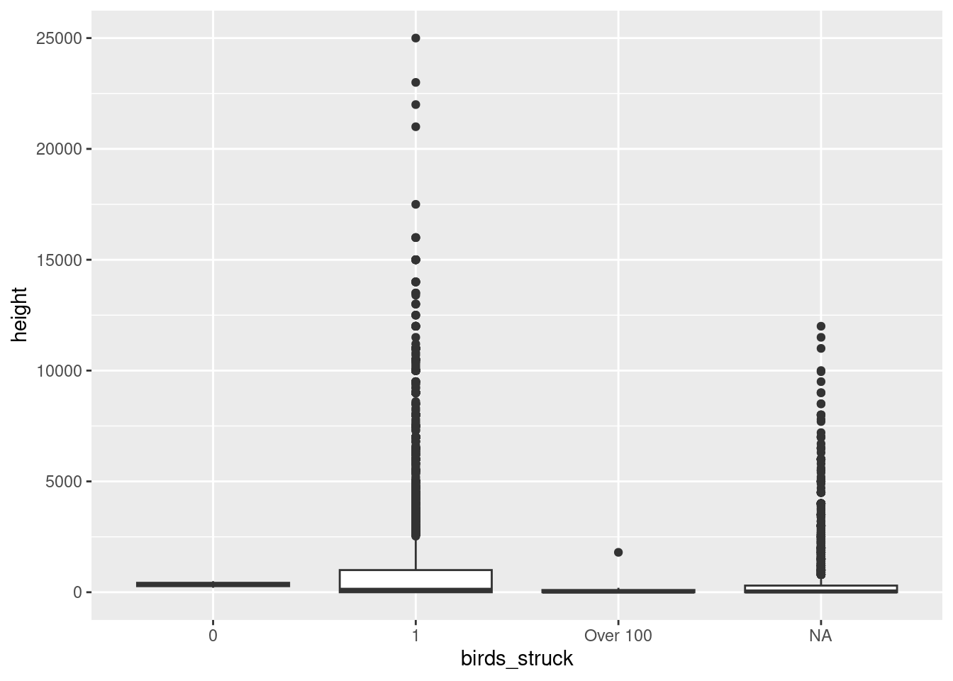
This project investigates bird strikes according to the time of day, phase of flight, number of birds struck, and aircraft height.

library(dplyr)
library(ggplot2)

dataset <- read.csv("../../../../data/birds_strikes.csv")

Data preparation

Four variables were selected for the analysis. Rows containing missing values or blank cells in these variables were removed before the analysis. After removing missing values and blank cells, 11,827 observations remained for the analysis.

subset <- dataset %>%
  select(time_of_day, phase_of_flt, birds_struck, height) %>%
  filter(
    !is.na(time_of_day),
    time_of_day != "",
    !is.na(phase_of_flt),
    phase_of_flt != "",
    !is.na(birds_struck),
    birds_struck != "",
    !is.na(height)
  )

Descriptive analysis

Bird strikes by time of day

subset %>%
  group_by(time_of_day)%>%
  summarise(count=n())

# A tibble: 4 × 2
  time_of_day count
  <chr>       <int>
1 Dawn          437
2 Day          7660
3 Dusk          595
4 Night        3135

ggplot(subset, aes(x = time_of_day)) +
  geom_bar()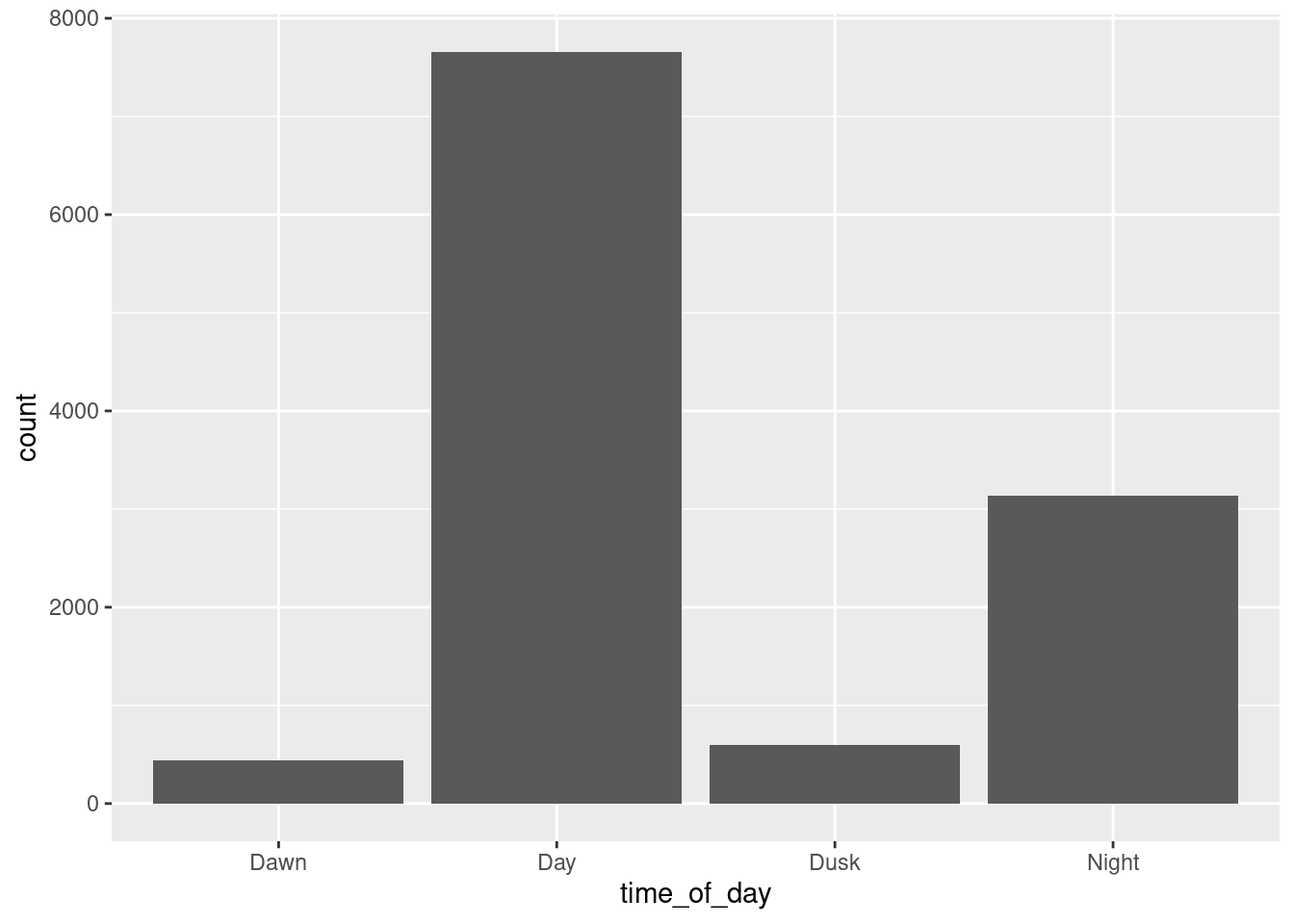

Bird strikes by phase of flight

The categories were reordered to reflect the typical sequence of a flight.

subset$phase_of_flt <- factor(
  subset$phase_of_flt,
  levels = c(
    "Take-off run",
    "Climb",
    "En Route",
    "Descent",
    "Approach",
    "Landing Roll",
    "Taxi",
    "Parked"
  )
)

subset |>
  group_by(phase_of_flt)|>
  summarise(count=n())

# A tibble: 8 × 2
  phase_of_flt count
  <fct>        <int>
1 Take-off run  1854
2 Climb         2453
3 En Route       331
4 Descent        461
5 Approach      4974
6 Landing Roll  1729
7 Taxi            19
8 Parked           6

ggplot(subset, aes(x = phase_of_flt)) +
  geom_bar()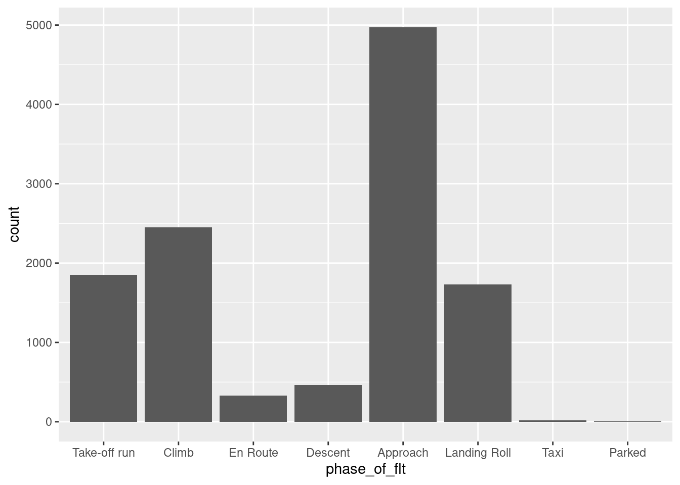

Birds strikes by number of birds struck

The categories are reordered in ascending order.

subset$birds_struck <- factor(
  subset$birds_struck,
  levels = c(
    "0",  
    "1",         
    "2 to 10",  
    "11 to 100", 
    "Over 100"  
  )
)

subset%>%
  group_by(birds_struck)%>%
  summarise(count=n())

# A tibble: 4 × 2
  birds_struck count
  <fct>        <int>
1 0                2
2 1             9090
3 Over 100        12
4 <NA>          2723

ggplot(subset, aes(x = birds_struck)) +
  geom_bar()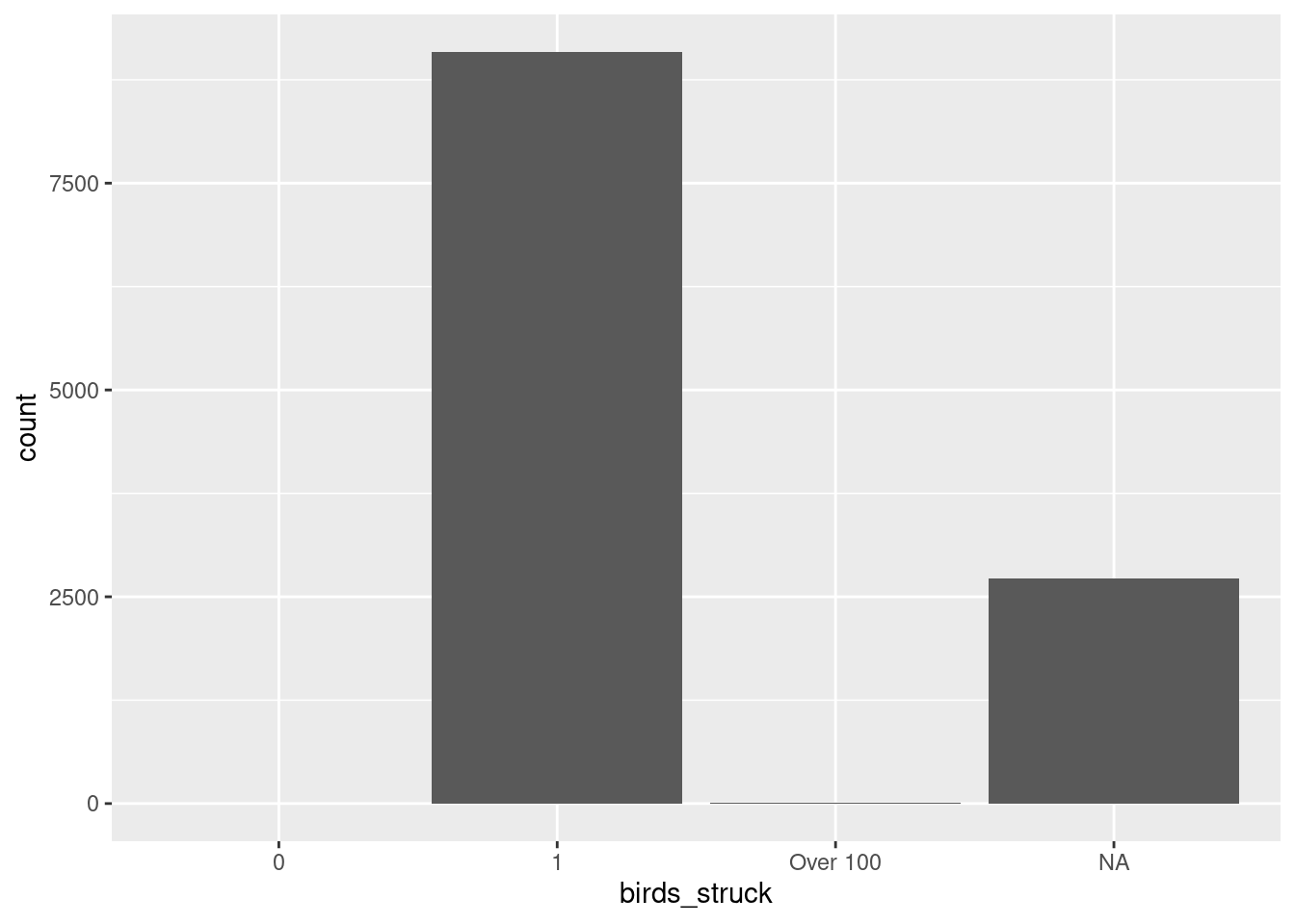

Height of bird strikes

summary(subset$height)

   Min. 1st Qu.  Median    Mean 3rd Qu.    Max. 
    0.0     0.0   100.0   889.8   900.0 25000.0 

ggplot(subset,
       aes(x=height))+
       geom_histogram()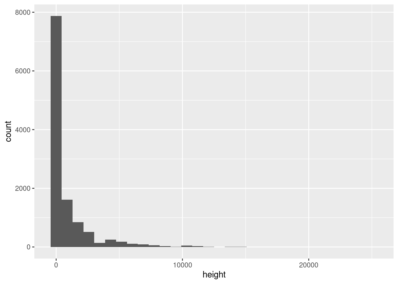

ggplot(subset,
       aes(y=height))+
       geom_boxplot()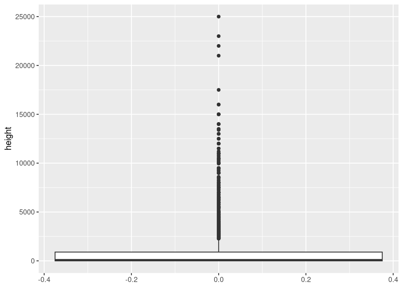

The distribution was strongly right-skewed, with a small number of observations at very high altitudes. The third quartile was 900 feet, indicating that 75% of bird strikes occurred at or below 900 feet. Therefore, a second histogram limited to 0–1,000 feet was produced to examine the distribution at lower altitudes more closely.

ggplot(subset,
       aes(x=height))+
       geom_histogram()+
       xlim(0,1000) +
       ylim(0,1500)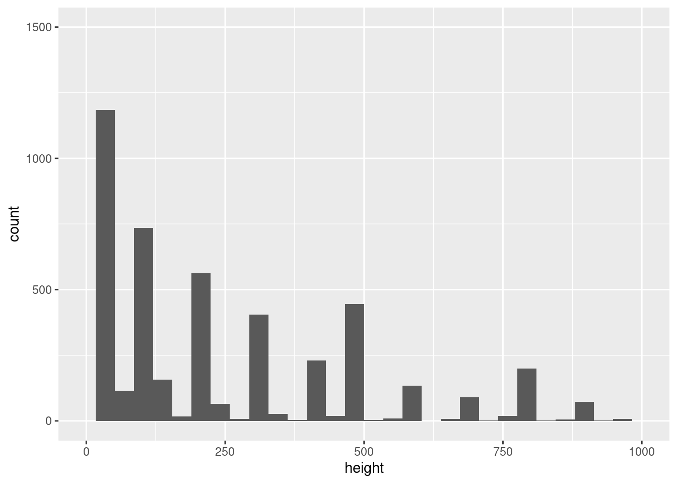   

Height and number of birds struck

ggplot(subset,
aes(x=birds_struck,
y=height))+
  geom_boxplot()